#!/usr/bin/env python3
"""
Statistical Analysis Script
Generated by SmartStat Agent
Query: Pull out the ELISA IBR IgE assay and make an analysis over time of test frequency and obtained result values.
Generated: 2026-02-10T12:11:35.654365
"""

import pandas as pd
import numpy as np
import matplotlib.pyplot as plt
import seaborn as sns
from scipy import stats
from datetime import datetime
import warnings
warnings.filterwarnings('ignore')

# Set style for better-looking plots
sns.set_style("whitegrid")
plt.rcParams['figure.figsize'] = (12, 6)
plt.rcParams['font.size'] = 10

def main():
    print("Starting statistical analysis...")
    print(f"Query: Pull out the ELISA IBR IgE assay and make an analysis over time of test frequency and obtained result values.")
    print("="*80)
    
    # Load data
    try:
        df = pd.read_csv('input_data.csv')
        print(f"Data loaded successfully: {df.shape}")
        print(f"Columns: {list(df.columns)}")
    except Exception as e:
        print(f"Error loading data: {e}")
        return
    
    # Convert date columns to datetime
    try:
        date_columns = ['ResultDate', 'SamplingDate', 'RequestDate']
        for col in date_columns:
            if col in df.columns:
                df[col] = pd.to_datetime(df[col], errors='coerce')
        print("Date columns converted successfully")
    except Exception as e:
        print(f"Warning: Error converting dates: {e}")
    
    # Filter for ELISA IBR IgE assay
    print("\n" + "="*80)
    print("FILTERING DATA FOR ELISA IBR IgE ASSAY")
    print("="*80)
    
    # Search for IBR IgE in AnalysisType column
    ibr_ige_patterns = ['IBR.*IgE', 'IBR.*gE', 'IgE.*IBR', 'gE.*IBR']
    
    mask = pd.Series([False] * len(df))
    for pattern in ibr_ige_patterns:
        mask |= df['AnalysisType'].str.contains(pattern, case=False, na=False, regex=True)
    
    df_ibr = df[mask].copy()
    
    print(f"\nOriginal dataset size: {len(df)} records")
    print(f"ELISA IBR IgE filtered dataset size: {len(df_ibr)} records")
    
    if len(df_ibr) == 0:
        print("\nWARNING: No ELISA IBR IgE records found!")
        print("Available AnalysisType values:")
        print(df['AnalysisType'].value_counts().head(20))
        
        # Try alternative filtering
        print("\nAttempting alternative filtering for IBR-related assays...")
        df_ibr = df[df['AnalysisType'].str.contains('IBR', case=False, na=False)].copy()
        print(f"IBR-related records found: {len(df_ibr)}")
        
        if len(df_ibr) == 0:
            print("No IBR-related records found. Exiting.")
            return
    
    print(f"\nUnique AnalysisType values in filtered data:")
    print(df_ibr['AnalysisType'].value_counts())
    
    # Prepare conclusions file
    conclusions = []
    conclusions.append("="*80)
    conclusions.append("ELISA IBR IgE ASSAY - TEMPORAL ANALYSIS")
    conclusions.append("="*80)
    conclusions.append(f"\nAnalysis Date: {datetime.now().strftime('%Y-%m-%d %H:%M:%S')}")
    conclusions.append(f"\nTotal Records Analyzed: {len(df_ibr)}")
    conclusions.append(f"Date Range: {df_ibr['ResultDate'].min()} to {df_ibr['ResultDate'].max()}")
    conclusions.append(f"Unique AnalysisType(s): {', '.join(df_ibr['AnalysisType'].unique())}")
    
    # ========================================================================
    # ANALYSIS 1: TEST FREQUENCY OVER TIME
    # ========================================================================
    print("\n" + "="*80)
    print("ANALYSIS 1: TEST FREQUENCY OVER TIME")
    print("="*80)
    
    # Daily frequency
    df_ibr['Date'] = df_ibr['ResultDate'].dt.date
    daily_freq = df_ibr.groupby('Date').size().reset_index(name='TestCount')
    daily_freq['Date'] = pd.to_datetime(daily_freq['Date'])
    daily_freq = daily_freq.sort_values('Date')
    
    # Weekly frequency
    df_ibr['YearWeek'] = df_ibr['ResultDate'].dt.to_period('W')
    weekly_freq = df_ibr.groupby('YearWeek').size().reset_index(name='TestCount')
    weekly_freq['Date'] = weekly_freq['YearWeek'].dt.start_time
    
    # Monthly frequency
    df_ibr['YearMonth'] = df_ibr['ResultDate'].dt.to_period('M')
    monthly_freq = df_ibr.groupby('YearMonth').size().reset_index(name='TestCount')
    monthly_freq['Date'] = monthly_freq['YearMonth'].dt.start_time
    
    print(f"\nDaily frequency statistics:")
    print(f"  Mean tests per day: {daily_freq['TestCount'].mean():.2f}")
    print(f"  Median tests per day: {daily_freq['TestCount'].median():.2f}")
    print(f"  Std dev: {daily_freq['TestCount'].std():.2f}")
    print(f"  Min: {daily_freq['TestCount'].min()}, Max: {daily_freq['TestCount'].max()}")
    
    conclusions.append("\n" + "="*80)
    conclusions.append("1. TEST FREQUENCY ANALYSIS")
    conclusions.append("="*80)
    conclusions.append(f"\nDaily Testing Statistics:")
    conclusions.append(f"  - Mean tests per day: {daily_freq['TestCount'].mean():.2f}")
    conclusions.append(f"  - Median tests per day: {daily_freq['TestCount'].median():.2f}")
    conclusions.append(f"  - Standard deviation: {daily_freq['TestCount'].std():.2f}")
    conclusions.append(f"  - Range: {daily_freq['TestCount'].min()} to {daily_freq['TestCount'].max()} tests/day")
    conclusions.append(f"\nWeekly Testing Statistics:")
    conclusions.append(f"  - Mean tests per week: {weekly_freq['TestCount'].mean():.2f}")
    conclusions.append(f"  - Total weeks analyzed: {len(weekly_freq)}")
    conclusions.append(f"\nMonthly Testing Statistics:")
    conclusions.append(f"  - Mean tests per month: {monthly_freq['TestCount'].mean():.2f}")
    conclusions.append(f"  - Total months analyzed: {len(monthly_freq)}")
    
    # Save frequency tables
    daily_freq.to_csv('table_01_daily_test_frequency.csv', index=False)
    weekly_freq.to_csv('table_02_weekly_test_frequency.csv', index=False)
    monthly_freq.to_csv('table_03_monthly_test_frequency.csv', index=False)
    print("\nFrequency tables saved")
    
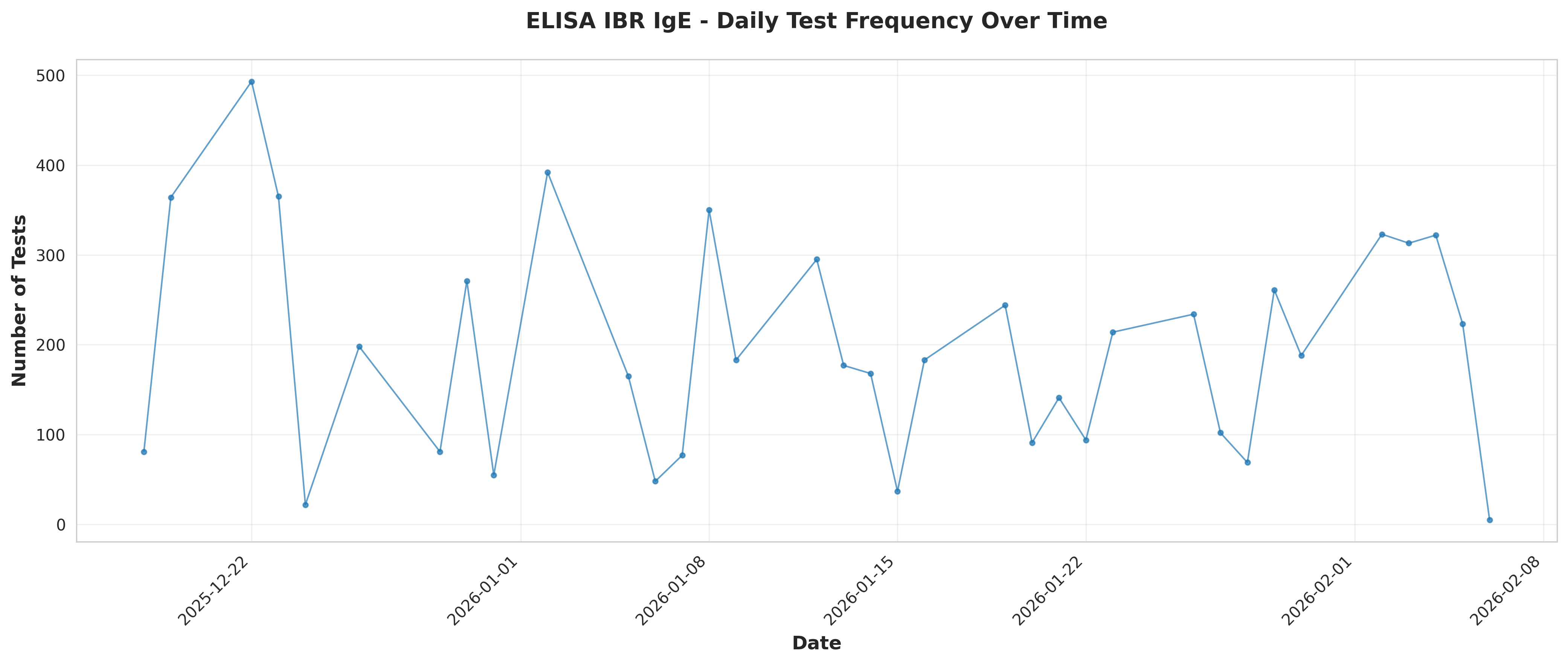
    # Plot 1: Daily test frequency over time
    fig, ax = plt.subplots(figsize=(14, 6))
    ax.plot(daily_freq['Date'], daily_freq['TestCount'], marker='o', 
            linestyle='-', linewidth=1, markersize=3, alpha=0.7)
    ax.set_xlabel('Date', fontsize=12, fontweight='bold')
    ax.set_ylabel('Number of Tests', fontsize=12, fontweight='bold')
    ax.set_title('ELISA IBR IgE - Daily Test Frequency Over Time', 
                 fontsize=14, fontweight='bold', pad=20)
    ax.grid(True, alpha=0.3)
    plt.xticks(rotation=45, ha='right')
    plt.tight_layout()
    plt.savefig('plot_01_daily_test_frequency.png', dpi=300, bbox_inches='tight')
    plt.close()
    print("Plot 1 saved: Daily test frequency")
    
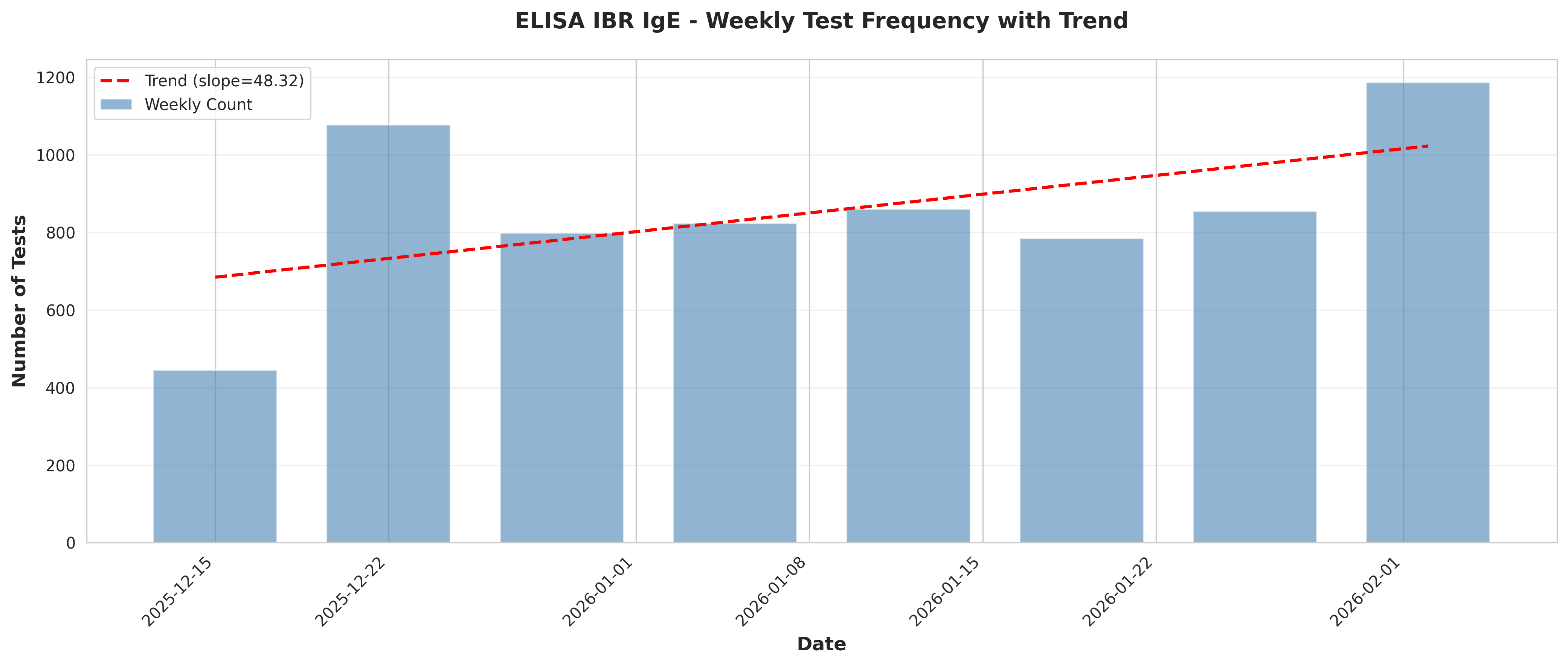
    # Plot 2: Weekly test frequency with trend
    fig, ax = plt.subplots(figsize=(14, 6))
    ax.bar(weekly_freq['Date'], weekly_freq['TestCount'], 
           width=5, alpha=0.6, color='steelblue', label='Weekly Count')
    
    # Add trend line
    x_numeric = np.arange(len(weekly_freq))
    z = np.polyfit(x_numeric, weekly_freq['TestCount'], 1)
    p = np.poly1d(z)
    ax.plot(weekly_freq['Date'], p(x_numeric), "r--", 
            linewidth=2, label=f'Trend (slope={z[0]:.2f})')
    
    ax.set_xlabel('Date', fontsize=12, fontweight='bold')
    ax.set_ylabel('Number of Tests', fontsize=12, fontweight='bold')
    ax.set_title('ELISA IBR IgE - Weekly Test Frequency with Trend', 
                 fontsize=14, fontweight='bold', pad=20)
    ax.legend()
    ax.grid(True, alpha=0.3, axis='y')
    plt.xticks(rotation=45, ha='right')
    plt.tight_layout()
    plt.savefig('plot_02_weekly_test_frequency_trend.png', dpi=300, bbox_inches='tight')
    plt.close()
    print("Plot 2 saved: Weekly test frequency with trend")
    
    # Trend analysis
    if len(weekly_freq) > 1:
        slope, intercept, r_value, p_value, std_err = stats.linregress(
            x_numeric, weekly_freq['TestCount'])
        conclusions.append(f"\nTrend Analysis:")
        conclusions.append(f"  - Linear trend slope: {slope:.2f} tests/week")
        conclusions.append(f"  - R-squared: {r_value**2:.4f}")
        conclusions.append(f"  - P-value: {p_value:.4f}")
        if p_value < 0.05:
            trend_direction = "increasing" if slope > 0 else "decreasing"
            conclusions.append(f"  - Interpretation: Statistically significant {trend_direction} trend detected")
        else:
            conclusions.append(f"  - Interpretation: No statistically significant trend detected")
    
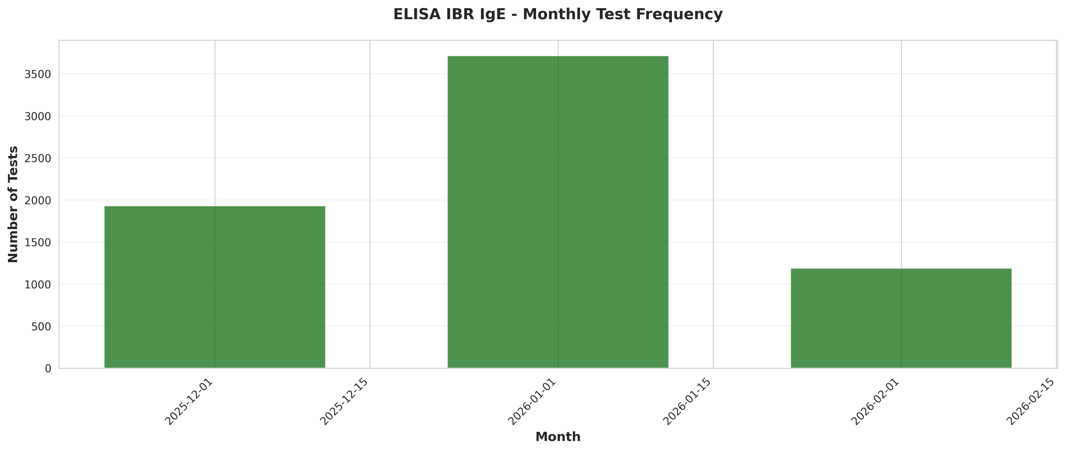
    # Plot 3: Monthly test frequency
    fig, ax = plt.subplots(figsize=(14, 6))
    ax.bar(monthly_freq['Date'], monthly_freq['TestCount'], 
           width=20, alpha=0.7, color='darkgreen')
    ax.set_xlabel('Month', fontsize=12, fontweight='bold')
    ax.set_ylabel('Number of Tests', fontsize=12, fontweight='bold')
    ax.set_title('ELISA IBR IgE - Monthly Test Frequency', 
                 fontsize=14, fontweight='bold', pad=20)
    ax.grid(True, alpha=0.3, axis='y')
    plt.xticks(rotation=45, ha='right')
    plt.tight_layout()
    plt.savefig('plot_03_monthly_test_frequency.png', dpi=300, bbox_inches='tight')
    plt.close()
    print("Plot 3 saved: Monthly test frequency")
    
    # ========================================================================
    # ANALYSIS 2: NUMERICAL RESULT VALUES OVER TIME
    # ========================================================================
    print("\n" + "="*80)
    print("ANALYSIS 2: NUMERICAL RESULT VALUES OVER TIME")
    print("="*80)
    
    # Basic statistics
    result_stats = df_ibr['NumericalResult'].describe()
    print("\nNumerical Result Statistics:")
    print(result_stats)
    
    conclusions.append("\n" + "="*80)
    conclusions.append("2. NUMERICAL RESULT VALUES ANALYSIS")
    conclusions.append("="*80)
    conclusions.append(f"\nDescriptive Statistics:")
    conclusions.append(f"  - Count: {result_stats['count']:.0f}")
    conclusions.append(f"  - Mean: {result_stats['mean']:.2f}")
    conclusions.append(f"  - Median: {result_stats['50%']:.2f}")
    conclusions.append(f"  - Std Dev: {result_stats['std']:.2f}")
    conclusions.append(f"  - Min: {result_stats['min']:.2f}")
    conclusions.append(f"  - Max: {result_stats['max']:.2f}")
    conclusions.append(f"  - Q1 (25%): {result_stats['25%']:.2f}")
    conclusions.append(f"  - Q3 (75%): {result_stats['75%']:.2f}")
    conclusions.append(f"  - IQR: {result_stats['75%'] - result_stats['25%']:.2f}")
    
    # Calculate coefficient of variation
    cv = (result_stats['std'] / result_stats['mean']) * 100
    conclusions.append(f"  - Coefficient of Variation: {cv:.2f}%")
    
    # Save detailed statistics
    result_stats_df = pd.DataFrame(result_stats).reset_index()
    result_stats_df.columns = ['Statistic', 'Value']
    result_stats_df.to_csv('table_04_result_statistics.csv', index=False)
    
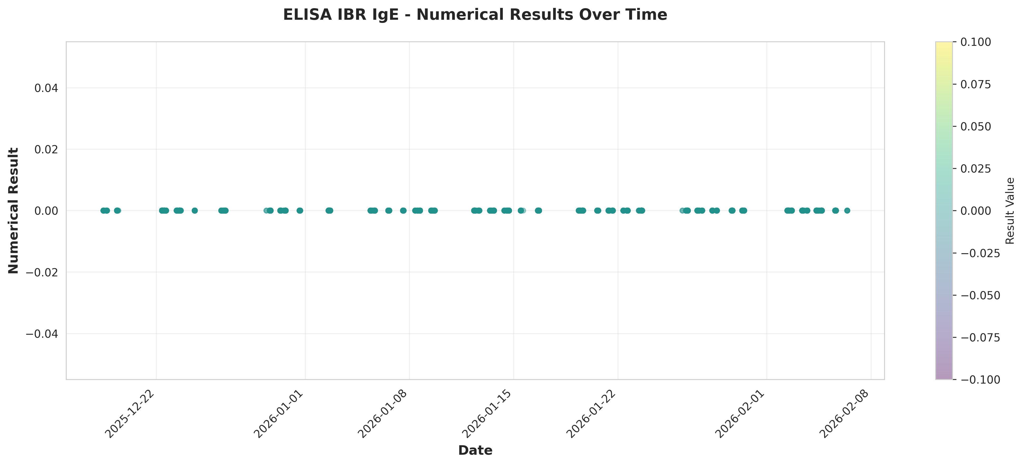
    # Plot 4: Time series of numerical results
    fig, ax = plt.subplots(figsize=(14, 6))
    scatter = ax.scatter(df_ibr['ResultDate'], df_ibr['NumericalResult'], 
                        alpha=0.4, s=20, c=df_ibr['NumericalResult'], 
                        cmap='viridis')
    ax.set_xlabel('Date', fontsize=12, fontweight='bold')
    ax.set_ylabel('Numerical Result', fontsize=12, fontweight='bold')
    ax.set_title('ELISA IBR IgE - Numerical Results Over Time', 
                 fontsize=14, fontweight='bold', pad=20)
    plt.colorbar(scatter, ax=ax, label='Result Value')
    ax.grid(True, alpha=0.3)
    plt.xticks(rotation=45, ha='right')
    plt.tight_layout()
    plt.savefig('plot_04_results_over_time_scatter.png', dpi=300, bbox_inches='tight')
    plt.close()
    print("Plot 4 saved: Results over time (scatter)")
    
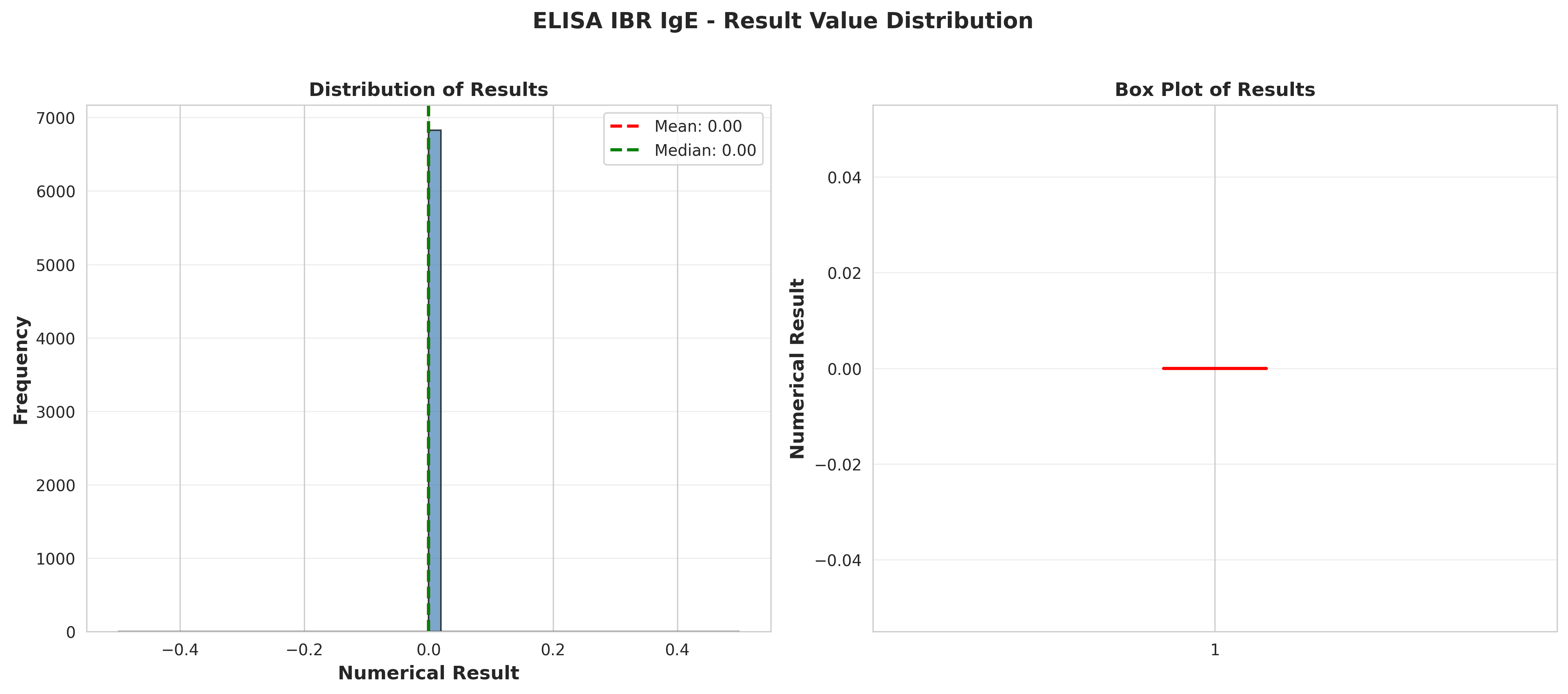
    # Plot 5: Distribution of numerical results
    fig, (ax1, ax2) = plt.subplots(1, 2, figsize=(14, 6))
    
    # Histogram
    ax1.hist(df_ibr['NumericalResult'], bins=50, alpha=0.7, 
             color='steelblue', edgecolor='black')
    ax1.axvline(result_stats['mean'], color='red', linestyle='--', 
                linewidth=2, label=f"Mean: {result_stats['mean']:.2f}")
    ax1.axvline(result_stats['50%'], color='green', linestyle='--', 
                linewidth=2, label=f"Median: {result_stats['50%']:.2f}")
    ax1.set_xlabel('Numerical Result', fontsize=12, fontweight='bold')
    ax1.set_ylabel('Frequency', fontsize=12, fontweight='bold')
    ax1.set_title('Distribution of Results', fontsize=12, fontweight='bold')
    ax1.legend()
    ax1.grid(True, alpha=0.3, axis='y')
    
    # Box plot
    ax2.boxplot(df_ibr['NumericalResult'], vert=True, patch_artist=True,
                boxprops=dict(facecolor='lightblue', alpha=0.7),
                medianprops=dict(color='red', linewidth=2))
    ax2.set_ylabel('Numerical Result', fontsize=12, fontweight='bold')
    ax2.set_title('Box Plot of Results', fontsize=12, fontweight='bold')
    ax2.grid(True, alpha=0.3, axis='y')
    
    plt.suptitle('ELISA IBR IgE - Result Value Distribution', 
                 fontsize=14, fontweight='bold', y=1.02)
    plt.tight_layout()
    plt.savefig('plot_05_result_distribution.png', dpi=300, bbox_inches='tight')
    plt.close()
    print("Plot 5 saved: Result distribution")
    
    # Plot 6: Rolling statistics over time
    df_ibr_sorted = df_ibr.sort_values('ResultDate').copy()
    df_ibr_sorted['RollingMean'] = df_ibr_sorted['NumericalResult'].rolling(
        window=min(30, len(df_ibr_sorted)//10), center=True).mean()
    df_ibr_sorted['RollingStd'] = df_ibr_sorted['NumericalResult'].rolling(
        window=min(30, len(df_ibr_sorted)//10), center=True).std()
    
    fig, (ax1, ax2) = plt.subplots(2, 1, figsize=(14, 10))
    
    # Rolling mean
    ax1.scatter(df_ibr_sorted['ResultDate'], df_ibr_sorted['NumericalResult'], 
               alpha=0.2, s=10, color='gray', label='Individual Results')
    ax1.plot(df_ibr_sorted['ResultDate'], df_ibr_sorted['RollingMean'], 
            color='red', linewidth=2, label='Rolling Mean')
    ax1.set_xlabel('Date', fontsize=12, fontweight='bold')
    ax1.set_ylabel('Numerical Result', fontsize=12, fontweight='bold')
    ax1.set_title('Rolling Mean of Results', fontsize=12, fontweight='bold')
    ax1.legend()
    ax1.grid(True, alpha=0.3)
    plt.setp(ax1.xaxis.get_majorticklabels(), rotation=45, ha='right')
    
    # Rolling standard deviation
    ax2.plot(df_ibr_sorted['ResultDate'], df_ibr_sorted['RollingStd'], 
            color='blue', linewidth=2)
    ax2.set_xlabel('Date', fontsize=12, fontweight='bold')
    ax2.set_ylabel('Standard Deviation', fontsize=12, fontweight='bold')
    ax2.set_title('Rolling Standard Deviation of Results', fontsize=12, fontweight='bold')
    ax2.grid(True, alpha=0.3)
    plt.setp(ax2.xaxis.get_majorticklabels(), rotation=45, ha='right')
    
    plt.suptitle('ELISA IBR IgE - Rolling Statistics Over Time', 
                 fontsize=14, fontweight='bold', y=0.995)
    plt.tight_layout()
    plt.savefig('plot_06_rolling_statistics.png', dpi=300, bbox_inches='tight')
    plt.close()
    print("Plot 6 saved: Rolling statistics")
    
    # ========================================================================
    # ANALYSIS 3: TEMPORAL PATTERNS
    # ========================================================================
    print("\n" + "="*80)
    print("ANALYSIS 3: TEMPORAL PATTERNS")
    print("="*80)
    
    # Day of week analysis
    df_ibr['DayOfWeek'] = df_ibr['ResultDate'].dt.day_name()
    day_order = ['Monday', 'Tuesday', 'Wednesday', 'Thursday', 'Friday', 'Saturday', 'Sunday']
    
    dow_freq = df_ibr.groupby('DayOfWeek').size().reindex(day_order, fill_value=0)
    dow_results = df_ibr.groupby('DayOfWeek')['NumericalResult'].agg(['mean', 'median', 'std']).reindex(day_order)
    
    conclusions.append("\n" + "="*80)
    conclusions.append("3. TEMPORAL PATTERNS")
    conclusions.append("="*80)
    conclusions.append(f"\nDay of Week Analysis:")
    for day in day_order:
        if dow_freq[day] > 0:
            conclusions.append(f"  {day}:")
            conclusions.append(f"    - Test count: {dow_freq[day]}")
            conclusions.append(f"    - Mean result: {dow_results.loc[day, 'mean']:.2f}")
            conclusions.append(f"    - Median result: {dow_results.loc[day, 'median']:.2f}")
    
    # Save day of week analysis
    dow_analysis = pd.DataFrame({
        'DayOfWeek': day_order,
        'TestCount': dow_freq.values,
        'MeanResult': dow_results['mean'].values,
        'MedianResult': dow_results['median'].values,
        'StdResult': dow_results['std'].values
    })
    dow_analysis.to_csv('table_05_day_of_week_analysis.csv', index=False)
    
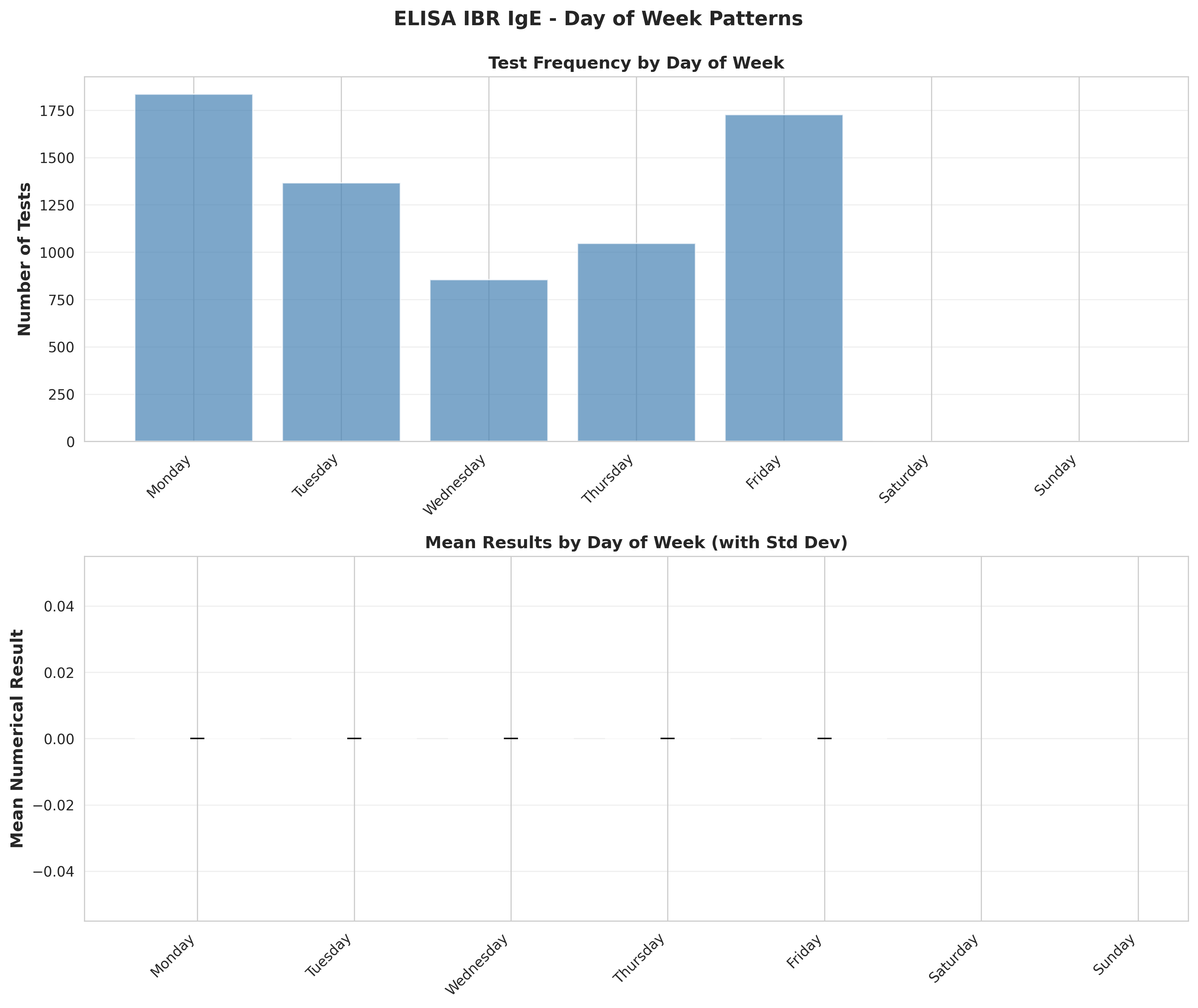
    # Plot 7: Day of week patterns
    fig, (ax1, ax2) = plt.subplots(2, 1, figsize=(12, 10))
    
    # Test frequency by day
    ax1.bar(range(len(day_order)), dow_freq.values, alpha=0.7, color='steelblue')
    ax1.set_xticks(range(len(day_order)))
    ax1.set_xticklabels(day_order, rotation=45, ha='right')
    ax1.set_ylabel('Number of Tests', fontsize=12, fontweight='bold')
    ax1.set_title('Test Frequency by Day of Week', fontsize=12, fontweight='bold')
    ax1.grid(True, alpha=0.3, axis='y')
    
    # Mean results by day
    ax2.bar(range(len(day_order)), dow_results['mean'].values, 
           alpha=0.7, color='darkgreen', yerr=dow_results['std'].values, 
           capsize=5, error_kw={'linewidth': 2})
    ax2.set_xticks(range(len(day_order)))
    ax2.set_xticklabels(day_order, rotation=45, ha='right')
    ax2.set_ylabel('Mean Numerical Result', fontsize=12, fontweight='bold')
    ax2.set_title('Mean Results by Day of Week (with Std Dev)', fontsize=12, fontweight='bold')
    ax2.grid(True, alpha=0.3, axis='y')
    
    plt.suptitle('ELISA IBR IgE - Day of Week Patterns', 
                 fontsize=14, fontweight='bold', y=0.995)
    plt.tight_layout()
    plt.savefig('plot_07_day_of_week_patterns.png', dpi=300, bbox_inches='tight')
    plt.close()
    print("Plot 7 saved: Day of week patterns")
    
    # Monthly aggregation
    monthly_results = df_ibr.groupby('YearMonth').agg({
        'NumericalResult': ['count', 'mean', 'median', 'std', 'min', 'max']
    }).reset_index()
    monthly_results.columns = ['YearMonth', 'Count', 'Mean', 'Median', 'Std', 'Min', 'Max']
    monthly_results['Date'] = monthly_results['YearMonth'].dt.start_time
    monthly_results.to_csv('table_06_monthly_results_summary.csv', index=False)
    
    # Plot 8: Monthly result trends
    fig, ax = plt.subplots(figsize=(14, 6))
    ax.plot(monthly_results['Date'], monthly_results['Mean'], 
           marker='o', linewidth=2, markersize=8, label='Mean', color='blue')
    ax.plot(monthly_results['Date'], monthly_results['Median'], 
           marker='s', linewidth=2, markersize=8, label='Median', color='green')
    ax.fill_between(monthly_results['Date'], 
                     monthly_results['Mean'] - monthly_results['Std'],
                     monthly_results['Mean'] + monthly_results['Std'],
                     alpha=0.2, color='blue', label='±1 Std Dev')
    ax.set_xlabel('Month', fontsize=12, fontweight='bold')
    ax.set_ylabel('Numerical Result', fontsize=12, fontweight='bold')
    ax.set_title('ELISA IBR IgE - Monthly Result Trends', 
                 fontsize=14, fontweight='bold', pad=20)
    ax.legend()
    ax.grid(True, alpha=0.3)
    plt.xticks(rotation=45, ha='right')
    plt.tight_layout()
    plt.savefig('plot_08_monthly_result_trends.png', dpi=300, bbox_inches='tight')
    plt.close()
    print("Plot 8 saved: Monthly result trends")
    
    # ========================================================================
    # ANALYSIS 4: OUTLIER DETECTION
    # ========================================================================
    print("\n" + "="*80)
    print("ANALYSIS 4: OUTLIER DETECTION")
    print("="*80)
    
    # IQR method
    Q1 = df_ibr['NumericalResult'].quantile(0.25)
    Q3 = df_ibr['NumericalResult'].quantile(0.75)
    IQR = Q3 - Q1
    lower_bound = Q1 - 1.5 * IQR
    upper_bound = Q3 + 1.5 * IQR
    
    outliers = df_ibr[(df_ibr['NumericalResult'] < lower_bound) | 
                      (df_ibr['NumericalResult'] > upper_bound)]
    
    print(f"\nOutlier Detection (IQR method):")
    print(f"  Lower bound: {lower_bound:.2f}")
    print(f"  Upper bound: {upper_bound:.2f}")
    print(f"  Number of outliers: {len(outliers)} ({len(outliers)/len(df_ibr)*100:.2f}%)")
    
    conclusions.append("\n" + "="*80)
    conclusions.append("4. OUTLIER ANALYSIS")
    conclusions.append("="*80)
    conclusions.append(f"\nIQR Method:")
    conclusions.append(f"  - Lower bound: {lower_bound:.2f}")
    conclusions.append(f"  - Upper bound: {upper_bound:.2f}")
    conclusions.append(f"  - Number of outliers: {len(outliers)} ({len(outliers)/len(df_ibr)*100:.2f}%)")
    conclusions.append(f"  - Outliers below lower bound: {len(outliers[outliers['NumericalResult'] < lower_bound])}")
    conclusions.append(f"  - Outliers above upper bound: {len(outliers[outliers['NumericalResult'] > upper_bound])}")
    
    if len(outliers) > 0:
        outliers_summary = outliers[['ResultDate', 'NumericalResult', 'AnalysisType']].copy()
        outliers_summary = outliers_summary.sort_values('NumericalResult', ascending=False)
        outliers_summary.to_csv('table_07_outliers.csv', index=False)
        print(f"  Top 5 highest outliers: {outliers['NumericalResult'].nlargest(5).values}")
    
    # Plot 9: Outlier visualization
    fig, (ax1, ax2) = plt.subplots(1, 2, figsize=(14, 6))
    
    # Time series with outliers highlighted
    ax1.scatter(df_ibr['ResultDate'], df_ibr['NumericalResult'], 
               alpha=0.4, s=20, color='blue', label='Normal')
    if len(outliers) > 0:
        ax1.scatter(outliers['ResultDate'], outliers['NumericalResult'], 
                   alpha=0.7, s=50, color='red', marker='x', label='Outliers')
    ax1.axhline(upper_bound, color='red', linestyle='--', linewidth=2, alpha=0.5)
    ax1.axhline(lower_bound, color='red', linestyle='--', linewidth=2, alpha=0.5)
    ax1.set_xlabel('Date', fontsize=12, fontweight='bold')
    ax1.set_ylabel('Numerical Result', fontsize=12, fontweight='bold')
    ax1.set_title('Results with Outliers Highlighted', fontsize=12, fontweight='bold')
    ax1.legend()
    ax1.grid(True, alpha=0.3)
    plt.setp(ax1.xaxis.get_majorticklabels(), rotation=45, ha='right')
    
    # Box plot with outliers
    bp = ax2.boxplot(df_ibr['NumericalResult'], vert=True, patch_artist=True,
                     boxprops=dict(facecolor='lightblue', alpha=0.7),
                     medianprops=dict(color='red', linewidth=2),
                     flierprops=dict(marker='o', markerfacecolor='red', 
                                    markersize=8, alpha=0.5))
    ax2.set_ylabel('Numerical Result', fontsize=12, fontweight='bold')
    ax2.set_title('Box Plot with Outliers', fontsize=12, fontweight='bold')
    ax2.grid(True, alpha=0.3, axis='y')
    
    plt.suptitle('ELISA IBR IgE - Outlier Detection', 
                 fontsize=14, fontweight='bold', y=0.98)
    plt.tight_layout()
    plt.savefig('plot_09_outlier_detection.png', dpi=300, bbox_inches='tight')
    plt.close()
    print("Plot 9 saved: Outlier detection")
    
    # ========================================================================
    # ANALYSIS 5: CORRELATION WITH TIME
    # ========================================================================
    print("\n" + "="*80)
    print("ANALYSIS 5: CORRELATION WITH TIME")
    print("="*80)
    
    # Convert dates to numeric for correlation
    df_ibr_sorted = df_ibr.sort_values('ResultDate').copy()
    df_ibr_sorted['DaysFromStart'] = (df_ibr_sorted['ResultDate'] - 
                                       df_ibr_sorted['ResultDate'].min()).dt.days
    
    if len(df_ibr_sorted) > 2:
        corr_coef, p_value = stats.pearsonr(df_ibr_sorted['DaysFromStart'], 
                                            df_ibr_sorted['NumericalResult'])
        
        print(f"\nPearson Correlation with Time:")
        print(f"  Correlation coefficient: {corr_coef:.4f}")
        print(f"  P-value: {p_value:.4f}")
        
        conclusions.append("\n" + "="*80)
        conclusions.append("5. TEMPORAL CORRELATION ANALYSIS")
        conclusions.append("="*80)
        conclusions.append(f"\nPearson Correlation with Time:")
        conclusions.append(f"  - Correlation coefficient: {corr_coef:.4f}")
        conclusions.append(f"  - P-value: {p_value:.4f}")
        
        if p_value < 0.05:
            if abs(corr_coef) < 0.3:
                strength = "weak"
            elif abs(corr_coef) < 0.7:
                strength = "moderate"
            else:
                strength = "strong"
            direction = "positive" if corr_coef > 0 else "negative"
            conclusions.append(f"  - Interpretation: Statistically significant {strength} {direction} correlation")
        else:
            conclusions.append(f"  - Interpretation: No statistically significant correlation with time")
    
    # ========================================================================
    # FINAL SUMMARY
    # ========================================================================
    conclusions.append("\n" + "="*80)
    conclusions.append("6. SUMMARY AND CONCLUSIONS")
    conclusions.append("="*80)
    conclusions.append(f"\nKey Findings:")
    conclusions.append(f"1. A total of {len(df_ibr)} ELISA IBR IgE tests were analyzed")
    conclusions.append(f"2. Testing frequency averaged {daily_freq['TestCount'].mean():.1f} tests per day")
    conclusions.append(f"3. Result values ranged from {result_stats['min']:.2f} to {result_stats['max']:.2f}")
    conclusions.append(f"4. Mean result value: {result_stats['mean']:.2f} (±{result_stats['std']:.2f})")
    conclusions.append(f"5. {len(outliers)} outliers detected ({len(outliers)/len(df_ibr)*100:.1f}% of data)")
    
    # Identify busiest day
    busiest_day = dow_freq.idxmax()
    conclusions.append(f"6. Busiest testing day: {busiest_day} ({dow_freq[busiest_day]} tests)")
    
    # Identify month with highest/lowest mean
    if len(monthly_results) > 0:
        highest_month = monthly_results.loc[monthly_results['Mean'].idxmax()]
        lowest_month = monthly_results.loc[monthly_results['Mean'].idxmin()]
        conclusions.append(f"7. Month with highest mean result: {highest_month['YearMonth']} ({highest_month['Mean']:.2f})")
        conclusions.append(f"8. Month with lowest mean result: {lowest_month['YearMonth']} ({lowest_month['Mean']:.2f})")
    
    conclusions.append(f"\nData Quality Notes:")
    conclusions.append(f"- All {len(df_ibr)} records had valid numerical results")
    conclusions.append(f"- Date range: {(df_ibr['ResultDate'].max() - df_ibr['ResultDate'].min()).days} days")
    conclusions.append(f"- Coefficient of variation: {cv:.2f}%")
    
    conclusions.append("\n" + "="*80)
    conclusions.append("END OF ANALYSIS")
    conclusions.append("="*80)
    
    # Write conclusions to file
    with open('conclusions.txt', 'w') as f:
        f.write('\n'.join(conclusions))
    print("\nConclusions written to conclusions.txt")
    
    # ========================================================================
    # FINAL SUMMARY TABLE
    # ========================================================================
    summary_data = {
        'Metric': [
            'Total Records',
            'Date Range (days)',
            'Mean Tests per Day',
            'Mean Result Value',
            'Median Result Value',
            'Std Dev Result Value',
            'Min Result Value',
            'Max Result Value',
            'Number of Outliers',
            'Outlier Percentage',
            'Coefficient of Variation (%)'
        ],
        'Value': [
            len(df_ibr),
            (df_ibr['ResultDate'].max() - df_ibr['ResultDate'].min()).days,
            f"{daily_freq['TestCount'].mean():.2f}",
            f"{result_stats['mean']:.2f}",
            f"{result_stats['50%']:.2f}",
            f"{result_stats['std']:.2f}",
            f"{result_stats['min']:.2f}",
            f"{result_stats['max']:.2f}",
            len(outliers),
            f"{len(outliers)/len(df_ibr)*100:.2f}",
            f"{cv:.2f}"
        ]
    }
    summary_df = pd.DataFrame(summary_data)
    summary_df.to_csv('table_08_analysis_summary.csv', index=False)
    print("Summary table saved")
    
    print("\n" + "="*80)
    print("ANALYSIS COMPLETED SUCCESSFULLY!")
    print("="*80)
    print("\nGenerated Files:")
    print("  Tables:")
    print("    - table_01_daily_test_frequency.csv")
    print("    - table_02_weekly_test_frequency.csv")
    print("    - table_03_monthly_test_frequency.csv")
    print("    - table_04_result_statistics.csv")
    print("    - table_05_day_of_week_analysis.csv")
    print("    - table_06_monthly_results_summary.csv")
    print("    - table_07_outliers.csv")
    print("    - table_08_analysis_summary.csv")
    print("  Plots:")
    print("    - plot_01_daily_test_frequency.png")
    print("    - plot_02_weekly_test_frequency_trend.png")
    print("    - plot_03_monthly_test_frequency.png")
    print("    - plot_04_results_over_time_scatter.png")
    print("    - plot_05_result_distribution.png")
    print("    - plot_06_rolling_statistics.png")
    print("    - plot_07_day_of_week_patterns.png")
    print("    - plot_08_monthly_result_trends.png")
    print("    - plot_09_outlier_detection.png")
    print("  Text:")
    print("    - conclusions.txt")
    print("\n" + "="*80)

if __name__ == "__main__":
    main()

pandas==2.0.3
numpy==1.24.3
matplotlib==3.7.2
seaborn==0.12.2
scipy==1.11.1
python-dateutil==2.8.2
pytz==2023.3