Session Info
test run
Status:
Completed
Progress
4 / 4 steps completed
Quick Actions
Dataset Overview
25000
Rows17
ColumnsColumn Types
Column Information
| Column | Type | Non-Null Count | Missing % | Unique Values |
|---|---|---|---|---|
| ResultId | int64 | 25000 | 0% | 25000 |
| ResultDate | datetime64[ns] | 25000 | 0% | 17779 |
| NumericalResult | float64 | 25000 | 0% | 4833 |
| Unit | float64 | 0 | 100.0% | 0 |
| ReferenceRange | float64 | 0 | 100.0% | 0 |
| AnalysisType | object | 25000 | 0% | 65 |
| AnalysisTypeNL | object | 25000 | 0% | 65 |
| AnalysisCode | object | 8966 | 64.1% | 26 |
| SampleNumber | object | 25000 | 0% | 15211 |
| SampleIdentification | object | 11710 | 53.2% | 8617 |
| SamplingDate | datetime64[ns] | 24809 | 0.8% | 88 |
| RequestNumber | int64 | 25000 | 0% | 980 |
| CustomerReference | object | 2162 | 91.4% | 97 |
| RequestDate | datetime64[ns] | 25000 | 0% | 980 |
| RequestOrigin | int64 | 25000 | 0% | 2 |
| TechValidated | bool | 25000 | 0% | 1 |
| BioValidated | bool | 25000 | 0% | 1 |
Generated SQL Query
Query length: 900
SELECT TOP 25000 res.Id AS ResultId, res.DateCreated AS ResultDate, res.Result_Value AS NumericalResult, res.Result_Unit AS Unit, res.Result_Reference AS ReferenceRange, a.Name_en AS AnalysisType, a.Name_nl AS AnalysisTypeNL, a.AnalyseCode AS AnalysisCode, s.SampleNr AS SampleNumber, s.Identification AS SampleIdentification, s.DateSampling AS SamplingDate, req.RequestNr AS RequestNumber, req.RefCustomer AS CustomerReference, req.DateCreated AS RequestDate, req.Ontvangstwijze AS RequestOrigin, res.TechValidated, res.BioValidated FROM Results res INNER JOIN Samples s ON res.Result_Sample = s.Id INNER JOIN Analyses a ON res.Result_Analysis = a.Id INNER JOIN Requests req ON s.Sample_Request = req.Id WHERE res.DateCreated >= DATEADD(MONTH, -3, GETDATE()) AND res.Result_Value IS NOT NULL AND res.TechValidated = 1 AND res.BioValidated = 1 ORDER BY res.DateCreated DESC, req.RequestNr, s.SampleNrAsk Your Question
Analysis History
Select for context:
Analysis 1
Pull out the ELISA IBR IgE assay and make an analysis over time of test frequency and obtained result values.
2026-02-10 12:14:04 • 20 files
Analysis 2
Descriptive statistics on the analysis type distribution in time and relative numbers.
2026-02-10 12:06:13 • 8 files
Debug: Found 20 generated files (1 scripts)
Generated Visualizations
Generated visualization
plot_02_weekly_test_frequency_trend.png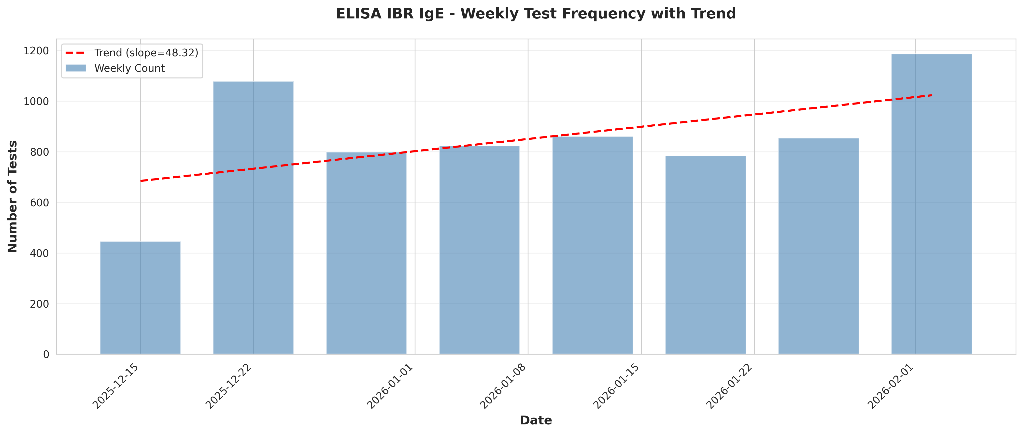
Generated visualization
plot_04_results_over_time_scatter.png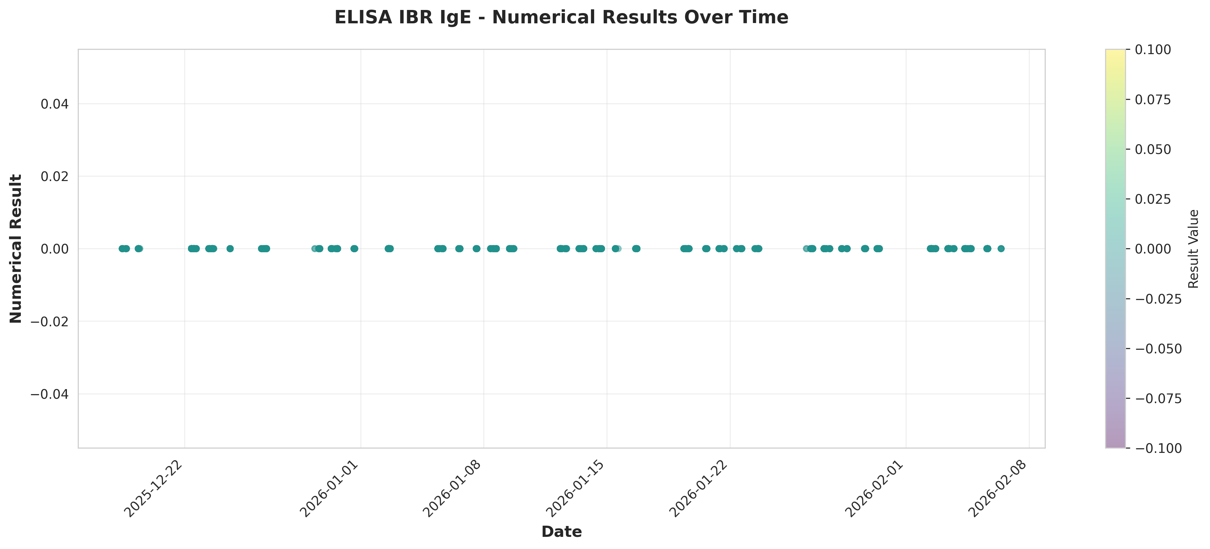
Generated visualization
plot_08_monthly_result_trends.png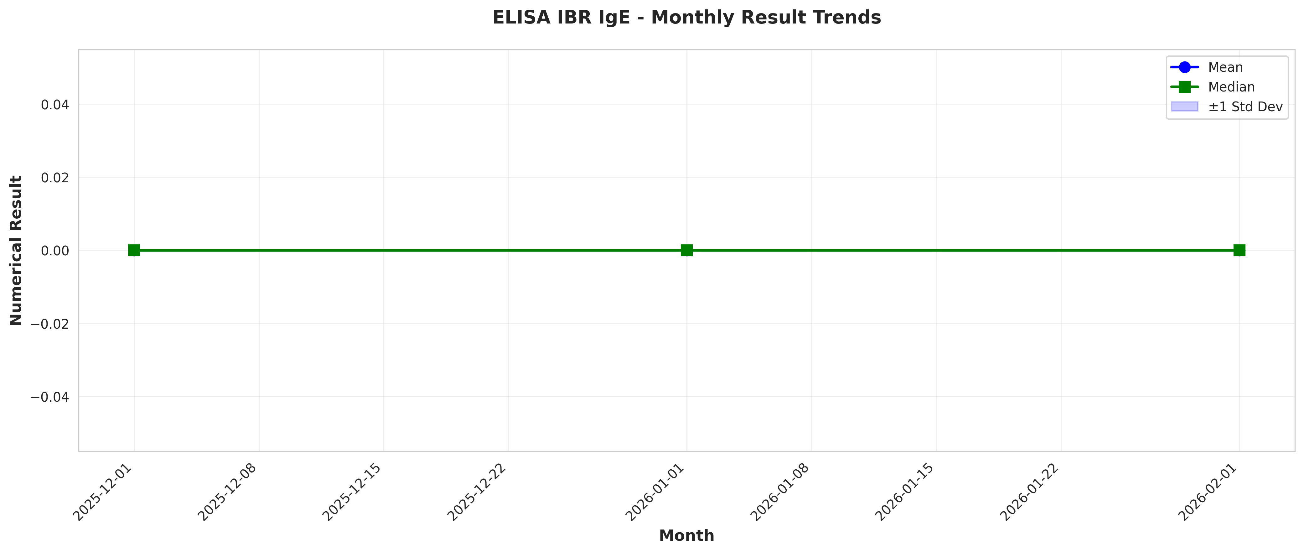
Generated visualization
plot_06_rolling_statistics.png
Generated visualization
plot_07_day_of_week_patterns.png
Generated visualization
plot_05_result_distribution.png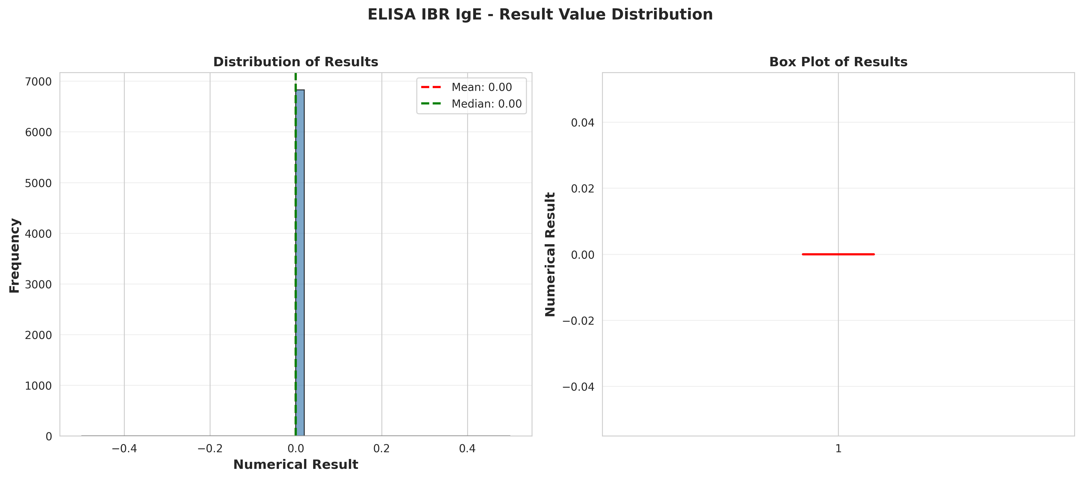
Generated visualization
plot_01_daily_test_frequency.png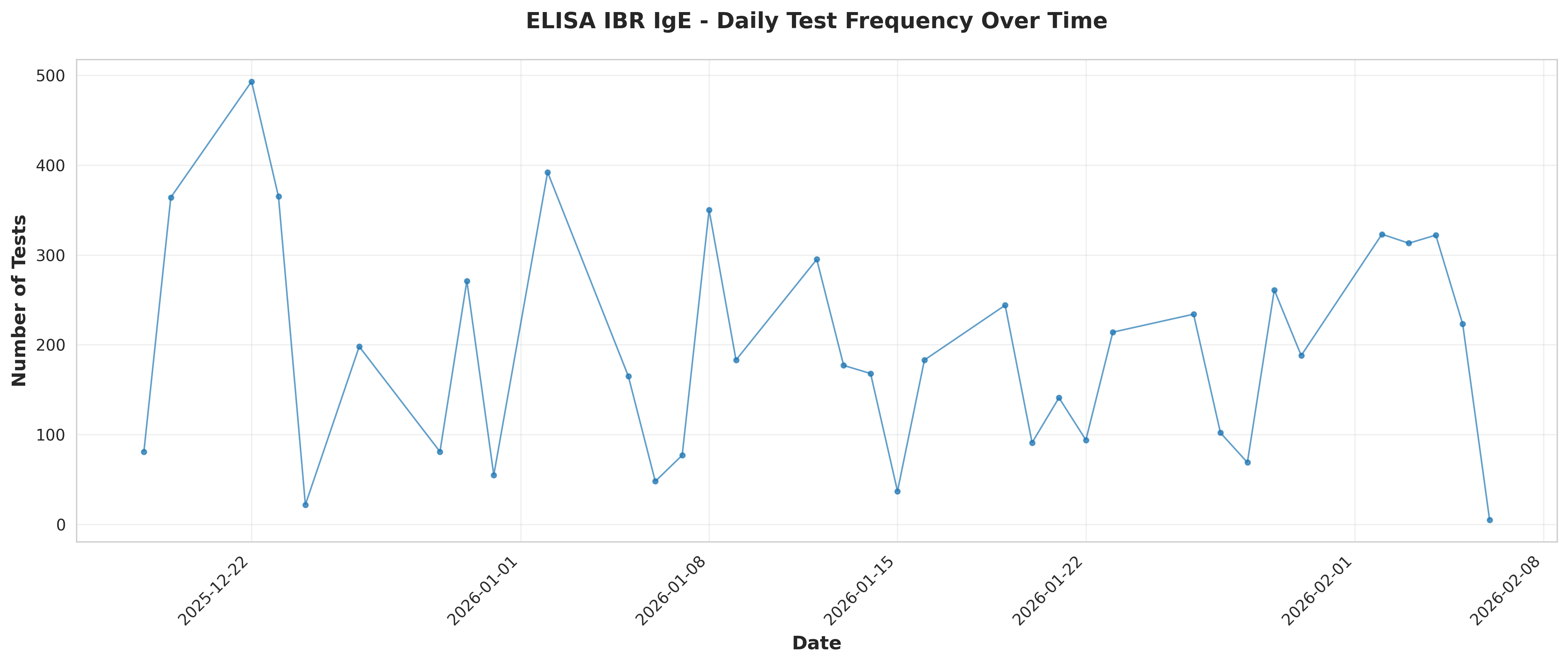
Generated visualization
plot_09_outlier_detection.png
Generated visualization
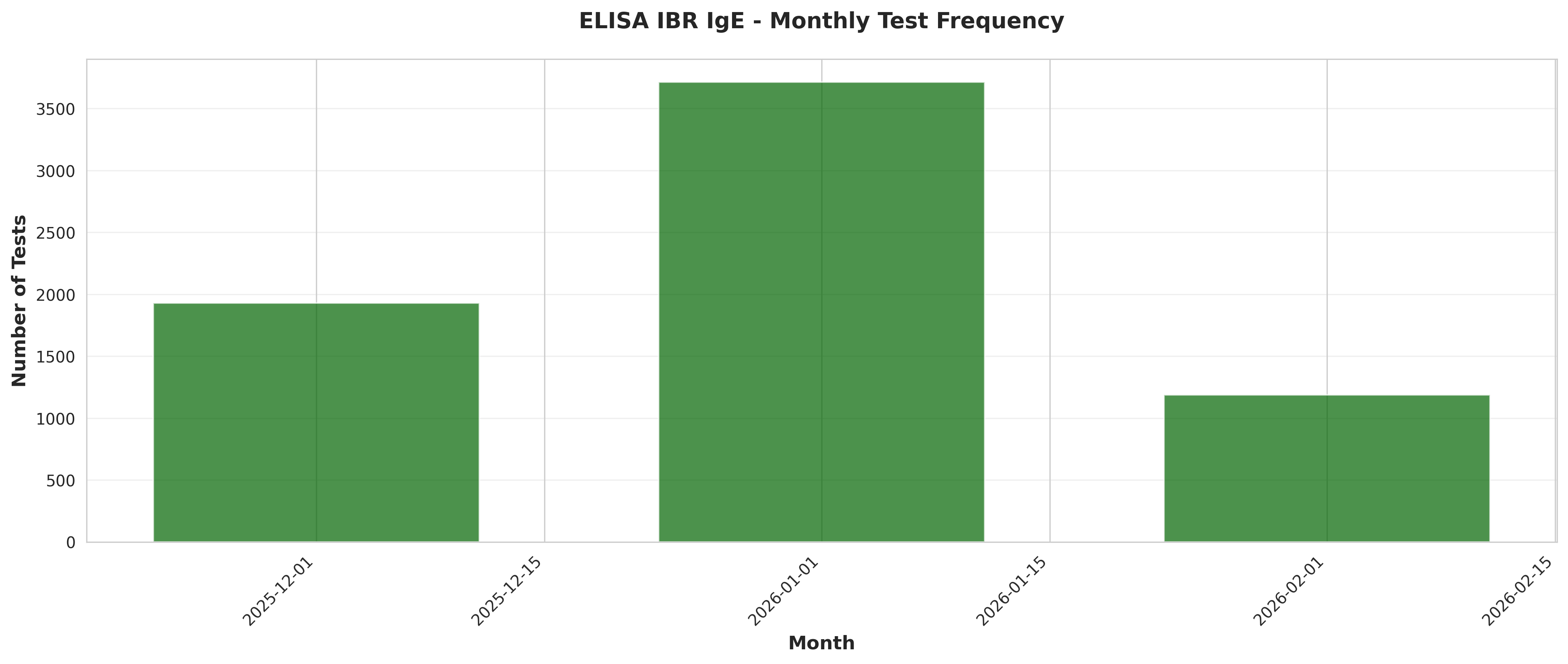
plot_03_monthly_test_frequency.png
Generated Tables
Data table or results
table_08_analysis_summary.csvMetric,Value Total Records,6829 Date Range (days),49 Mean Tests per Day,195.11 Mean Result Value,0.00 Median Result Value,0.00 Std Dev Result Value,0.00 Min Result Value,0.00 Max Result Value,0.00 Number of Outliers,0 Outlier Percentage,0.00 Coefficient of Variation (%),nan
Data table or results
table_02_weekly_test_frequency.csvYearWeek,TestCount,Date 2025-12-15/2025-12-21,445,2025-12-15 2025-12-22/2025-12-28,1078,2025-12-22 2025-12-29/2026-01-04,799,2025-12-29 2026-01-05/2026-01-11,823,2026-01-05 2026-01-12/2026-01-18,860,2026-01-12 2026-01-19/2026-01-25,784,2026-01-19 2026-01-26/2026-02-01,854,2026-01-26 2026-02-02/2026-02-08,1186,2026-02-02
Data table or results
input_data.csvResultId,ResultDate,NumericalResult,Unit,ReferenceRange,AnalysisType,AnalysisTypeNL,AnalysisCode,SampleNumber,SampleIdentification,SamplingDate,RequestNumber,CustomerReference,RequestDate,RequestOrigin,TechValidated,BioValidated 3034907,2026-02-09 16:58:05.000,1.0,,,Ascaridia/ Heterakis,Ascaridia/ Heterakis,Asc/Het,656293/1,Fiente,2026-01-22,656293,,2026-02-09 11:18:10,2,True,True 3034909,2026-02-09 16:58:05.000,0.0,,,Trichostrongylus,Trichostrongylus,Trich,656293/1,Fiente,2026-01-22,656293,,202...
Data table or results
table_05_day_of_week_analysis.csvDayOfWeek,TestCount,MeanResult,MedianResult,StdResult Monday,1835,0.0,0.0,0.0 Tuesday,1367,0.0,0.0,0.0 Wednesday,854,0.0,0.0,0.0 Thursday,1046,0.0,0.0,0.0 Friday,1727,0.0,0.0,0.0 Saturday,0,,, Sunday,0,,,
Data table or results
table_06_monthly_results_summary.csvYearMonth,Count,Mean,Median,Std,Min,Max,Date 2025-12,1930,0.0,0.0,0.0,0.0,0.0,2025-12-01 2026-01,3713,0.0,0.0,0.0,0.0,0.0,2026-01-01 2026-02,1186,0.0,0.0,0.0,0.0,0.0,2026-02-01
Data table or results
table_04_result_statistics.csvStatistic,Value count,6829.0 mean,0.0 std,0.0 min,0.0 25%,0.0 50%,0.0 75%,0.0 max,0.0
Data table or results
table_03_monthly_test_frequency.csvYearMonth,TestCount,Date 2025-12,1930,2025-12-01 2026-01,3713,2026-01-01 2026-02,1186,2026-02-01
Data table or results
table_01_daily_test_frequency.csvDate,TestCount 2025-12-18,81 2025-12-19,364 2025-12-22,493 2025-12-23,365 2025-12-24,22 2025-12-26,198 2025-12-29,81 2025-12-30,271 2025-12-31,55 2026-01-02,392 2026-01-05,165 2026-01-06,48 2026-01-07,77 2026-01-08,350 2026-01-09,183 2026-01-12,295 2026-01-13,177 2026-01-14,168 2026-01-15,37 2026-01-16,183 2026-01-19,244 2026-01-20,91 2026-01-21,141 2026-01-22,94 2026-01-23,214 2026-01-26,234 2026-01-27,102 2026-01-28,69 2026-01-29,261 2026-01-30,188 2026-02-02,323 2026-02-03,313 2026-02-04,322 ...
Analysis Conclusions
Analysis conclusions and insights
conclusions.txt
================================================================================
ELISA IBR IgE ASSAY - TEMPORAL ANALYSIS
================================================================================
Analysis Date: 2026-02-10 12:13:48
Total Records Analyzed: 6829
Date Range: 2025-12-18 10:46:47 to 2026-02-06 09:48:14
Unique AnalysisType(s): ELISA IBR gE (B)
================================================================================
1. TEST FREQUENCY ANALYSIS
================================================================================
Daily Testing Statistics:
- Mean tests per day: 195.11
- Median tests per day: 183.00
- Standard deviation: 121.70
- Range: 5 to 493 tests/day
Weekly Testing Statistics:
- Mean tests per week: 853.62
- Total weeks analyzed: 8
Monthly Testing Statistics:
- Mean tests per month: 2276.33
- Total months analyzed: 3
Trend Analysis:
- Linear trend slope: 48.32 tests/week
- R-squared: 0.2913
- P-value: 0.1673
- Interpretation: No statistically significant trend detected
================================================================================
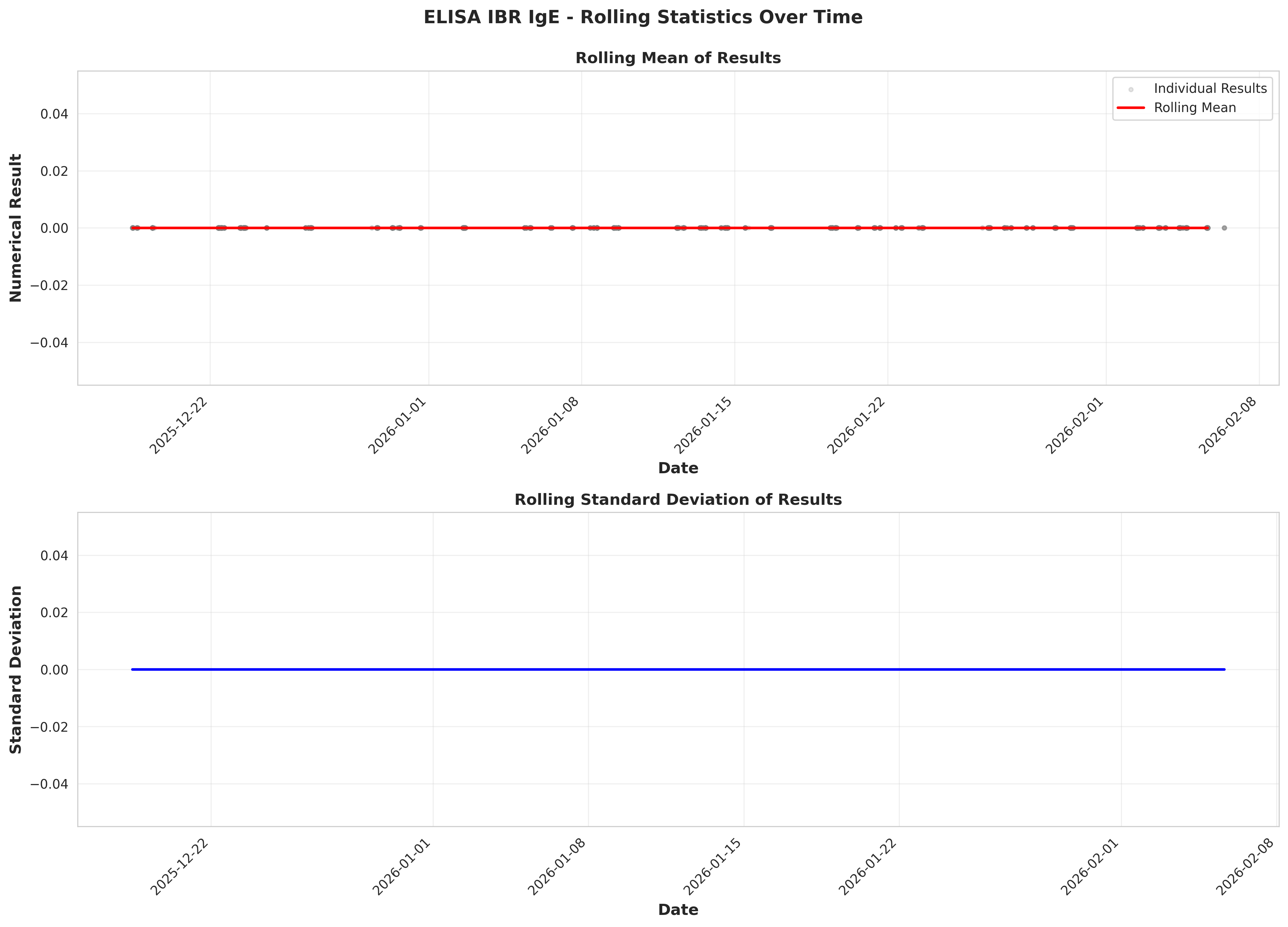
2. NUMERICAL RESULT VALUES ANALYSIS
================================================================================
Descriptive Statistics:
- Count: 6829
- Mean: 0.00
- Median: 0.00
- Std Dev: 0.00
- Min: 0.00
- Max: 0.00
- Q1 (25%): 0.00
- Q3 (75%): 0.00
- IQR: 0.00
- Coefficient of Variation: nan%
================================================================================
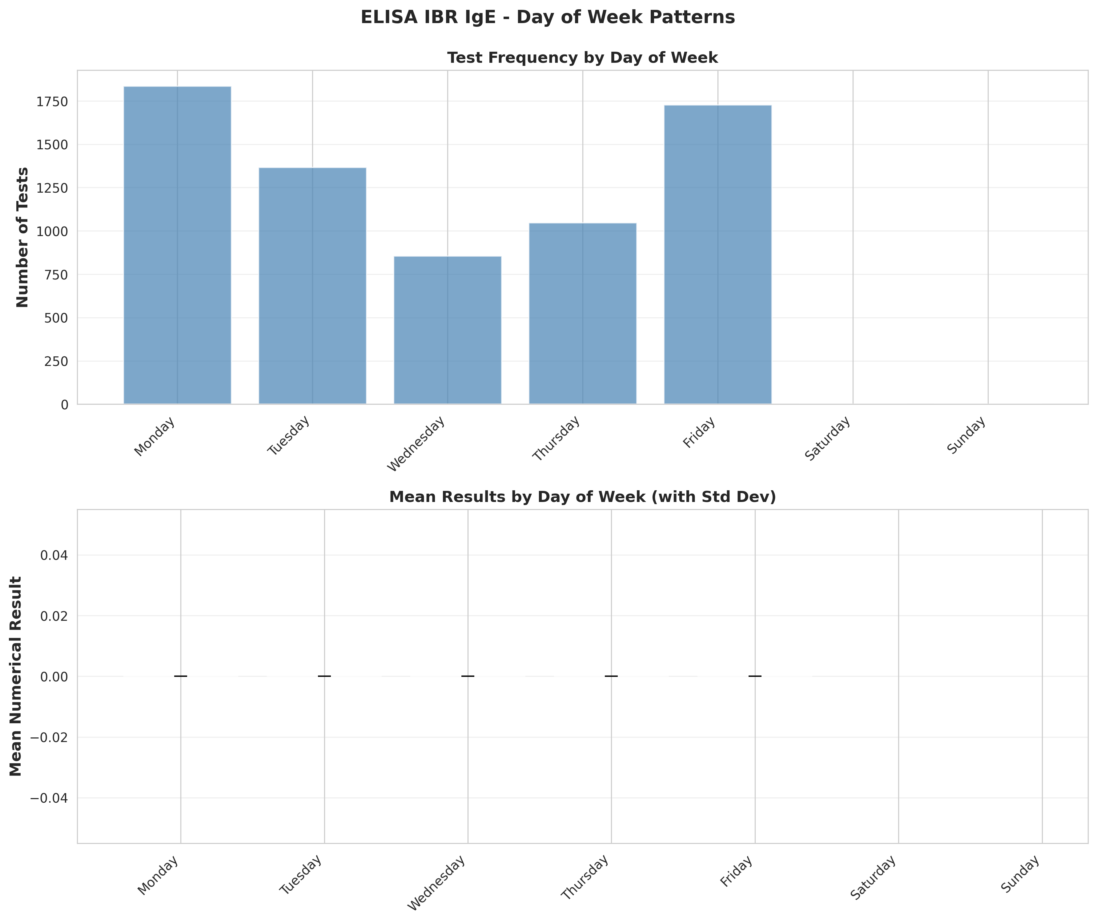
3. TEMPORAL PATTERNS
================================================================================
Day of Week Analysis:
Monday:
- Test count: 1835
- Mean result: 0.00
- Median result: 0.00
Tuesday:
- Test count: 1367
- Mean result: 0.00
- Median result: 0.00
Wednesday:
- Test count: 854
- Mean result: 0.00
- Median result: 0.00
Thursday:
- Test count: 1046
- Mean result: 0.00
- Median result: 0.00
ELISA IBR IgE ASSAY - TEMPORAL ANALYSIS
================================================================================
Analysis Date: 2026-02-10 12:13:48
Total Records Analyzed: 6829
Date Range: 2025-12-18 10:46:47 to 2026-02-06 09:48:14
Unique AnalysisType(s): ELISA IBR gE (B)
================================================================================
1. TEST FREQUENCY ANALYSIS
================================================================================
Daily Testing Statistics:
- Mean tests per day: 195.11
- Median tests per day: 183.00
- Standard deviation: 121.70
- Range: 5 to 493 tests/day
Weekly Testing Statistics:
- Mean tests per week: 853.62
- Total weeks analyzed: 8
Monthly Testing Statistics:
- Mean tests per month: 2276.33
- Total months analyzed: 3
Trend Analysis:
- Linear trend slope: 48.32 tests/week
- R-squared: 0.2913
- P-value: 0.1673
- Interpretation: No statistically significant trend detected
================================================================================
2. NUMERICAL RESULT VALUES ANALYSIS
================================================================================
Descriptive Statistics:
- Count: 6829
- Mean: 0.00
- Median: 0.00
- Std Dev: 0.00
- Min: 0.00
- Max: 0.00
- Q1 (25%): 0.00
- Q3 (75%): 0.00
- IQR: 0.00
- Coefficient of Variation: nan%
================================================================================
3. TEMPORAL PATTERNS
================================================================================
Day of Week Analysis:
Monday:
- Test count: 1835
- Mean result: 0.00
- Median result: 0.00
Tuesday:
- Test count: 1367
- Mean result: 0.00
- Median result: 0.00
Wednesday:
- Test count: 854
- Mean result: 0.00
- Median result: 0.00
Thursday:
- Test count: 1046
- Mean result: 0.00
- Median result: 0.00
Generated Scripts
Generated Python analysis script
analysis.py
Content length: 29521
#!/usr/bin/env python3
"""
Statistical Analysis Script
Generated by SmartStat Agent
Query: Pull out the ELISA IBR IgE assay and make an analysis over time of test frequency and obtained result values.
Generated: 2026-02-10T12:11:35.654365
"""
import pandas as pd
import numpy as np
import matplotlib.pyplot as plt
import seaborn as sns
from scipy import stats
from datetime import datetime
import warnings
warnings.filterwarnings('ignore')
# Set style for better-looking plots
sns.set_style("whitegrid")
plt.rcParams['figure.figsize'] = (12, 6)
plt.rcParams['font.size'] = 10
def main():
print("Starting statistical analysis...")
print(f"Query: Pull out the ELISA IBR IgE assay and make an analysis over time of test frequency and obtained result values.")
print("="*80)
# Load data
try:
df = pd.read_csv('input_data.csv')
print(f"Data loaded successfully: {df.shape}")
print(f"Columns: {list(df.columns)}")
except Exception as e:
print(f"Error loading data: {e}")
return
# Convert date columns to datetime
try:
date_columns = ['ResultDate', 'SamplingDate', 'RequestDate']
for col in date_columns:
if col in df.columns:
df[col] = pd.to_datetime(df[col], errors='coerce')
print("Date columns converted successfully")
except Exception as e:
print(f"Warning: Error converting dates: {e}")
# Filter for ELISA IBR IgE assay
print("\n" + "="*80)
print("FILTERING DATA FOR ELISA IBR IgE ASSAY")
print("="*80)
# Search for IBR IgE in AnalysisType column
ibr_ige_patterns = ['IBR.*IgE', 'IBR.*gE', 'IgE.*IBR', 'gE.*IBR']
mask = pd.Series([False] * len(df))
for pattern in ibr_ige_patterns:
mask |= df['AnalysisType'].str.contains(pattern, case=False, na=False, regex=True)
df_ibr = df[mask].copy()
print(f"\nOriginal dataset size: {len(df)} records")
print(f"ELISA IBR IgE filtered dataset size: {len(df_ibr)} records")
if len(df_ibr) == 0:
print("\nWARNING: No ELISA IBR IgE records found!")
print("Available AnalysisType values:")
print(df['AnalysisType'].value_counts().head(20))
# Try alternative filtering
print("\nAttempting alternative filtering for IBR-related assays...")
df_ibr = df[df['AnalysisType'].str.contains('IBR', case=False, na=False)].copy()
print(f"IBR-related records found: {len(df_ibr)}")
if len(df_ibr) == 0:
print("No IBR-related records found. Exiting.")
return
print(f"\nUnique AnalysisType values in filtered data:")
print(df_ibr['AnalysisType'].value_counts())
# Prepare conclusions file
conclusions = []
conclusions.append("="*80)
conclusions.append("ELISA IBR IgE ASSAY - TEMPORAL ANALYSIS")
conclusions.append("="*80)
conclusions.append(f"\nAnalysis Date: {datetime.now().strftime('%Y-%m-%d %H:%M:%S')}")
conclusions.append(f"\nTotal Records Analyzed: {len(df_ibr)}")
conclusions.append(f"Date Range: {df_ibr['ResultDate'].min()} to {df_ibr['ResultDate'].max()}")
conclusions.append(f"Unique AnalysisType(s): {', '.join(df_ibr['AnalysisType'].unique())}")
# ========================================================================
# ANALYSIS 1: TEST FREQUENCY OVER TIME
# ========================================================================
print("\n" + "="*80)
print("ANALYSIS 1: TEST FREQUENCY OVER TIME")
print("="*80)
# Daily frequency
df_ibr['Date'] = df_ibr['ResultDate'].dt.date
daily_freq = df_ibr.groupby('Date').size().reset_index(name='TestCount')
daily_freq['Date'] = pd.to_datetime(daily_freq['Date'])
daily_freq = daily_freq.sort_values('Date')
# Weekly frequency
df_ibr['YearWeek'] = df_ibr['ResultDate'].dt.to_period('W')
weekly_freq = df_ibr.groupby('YearWeek').size().reset_index(name='TestCount')
weekly_freq['Date'] = weekly_freq['YearWeek'].dt.start_time
# Monthly frequency
df_ibr['YearMonth'] = df_ibr['ResultDate'].dt.to_period('M')
monthly_freq = df_ibr.groupby('YearMonth').size().reset_index(name='TestCount')
monthly_freq['Date'] = monthly_freq['YearMonth'].dt.start_time
print(f"\nDaily frequency statistics:")
print(f" Mean tests per day: {daily_freq['TestCount'].mean():.2f}")
print(f" Median tests per day: {daily_freq['TestCount'].median():.2f}")
print(f" Std dev: {daily_freq['TestCount'].std():.2f}")
print(f" Min: {daily_freq['TestCount'].min()}, Max: {daily_freq['TestCount'].max()}")
conclusions.append("\n" + "="*80)
conclusions.append("1. TEST FREQUENCY ANALYSIS")
conclusions.append("="*80)
conclusions.append(f"\nDaily Testing Statistics:")
conclusions.append(f" - Mean tests per day: {daily_freq['TestCount'].mean():.2f}")
conclusions.append(f" - Median tests per day: {daily_freq['TestCount'].median():.2f}")
conclusions.append(f" - Standard deviation: {daily_freq['TestCount'].std():.2f}")
conclusions.append(f" - Range: {daily_freq['TestCount'].min()} to {daily_freq['TestCount'].max()} tests/day")
conclusions.append(f"\nWeekly Testing Statistics:")
conclusions.append(f" - Mean tests per week: {weekly_freq['TestCount'].mean():.2f}")
conclusions.append(f" - Total weeks analyzed: {len(weekly_freq)}")
conclusions.append(f"\nMonthly Testing Statistics:")
conclusions.append(f" - Mean tests per month: {monthly_freq['TestCount'].mean():.2f}")
conclusions.append(f" - Total months analyzed: {len(monthly_freq)}")
# Save frequency tables
daily_freq.to_csv('table_01_daily_test_frequency.csv', index=False)
weekly_freq.to_csv('table_02_weekly_test_frequency.csv', index=False)
monthly_freq.to_csv('table_03_monthly_test_frequency.csv', index=False)
print("\nFrequency tables saved")
# Plot 1: Daily test frequency over time
fig, ax = plt.subplots(figsize=(14, 6))
ax.plot(daily_freq['Date'], daily_freq['TestCount'], marker='o',
linestyle='-', linewidth=1, markersize=3, alpha=0.7)
ax.set_xlabel('Date', fontsize=12, fontweight='bold')
ax.set_ylabel('Number of Tests', fontsize=12, fontweight='bold')
ax.set_title('ELISA IBR IgE - Daily Test Frequency Over Time',
fontsize=14, fontweight='bold', pad=20)
ax.grid(True, alpha=0.3)
plt.xticks(rotation=45, ha='right')
plt.tight_layout()
plt.savefig('plot_01_daily_test_frequency.png', dpi=300, bbox_inches='tight')
plt.close()
print("Plot 1 saved: Daily test frequency")
# Plot 2: Weekly test frequency with trend
fig, ax = plt.subplots(figsize=(14, 6))
ax.bar(weekly_freq['Date'], weekly_freq['TestCount'],
width=5, alpha=0.6, color='steelblue', label='Weekly Count')
# Add trend line
x_numeric = np.arange(len(weekly_freq))
z = np.polyfit(x_numeric, weekly_freq['TestCount'], 1)
p = np.poly1d(z)
ax.plot(weekly_freq['Date'], p(x_numeric), "r--",
linewidth=2, label=f'Trend (slope={z[0]:.2f})')
ax.set_xlabel('Date', fontsize=12, fontweight='bold')
ax.set_ylabel('Number of Tests', fontsize=12, fontweight='bold')
ax.set_title('ELISA IBR IgE - Weekly Test Frequency with Trend',
fontsize=14, fontweight='bold', pad=20)
ax.legend()
ax.grid(True, alpha=0.3, axis='y')
plt.xticks(rotation=45, ha='right')
plt.tight_layout()
plt.savefig('plot_02_weekly_test_frequency_trend.png', dpi=300, bbox_inches='tight')
plt.close()
print("Plot 2 saved: Weekly test frequency with trend")
# Trend analysis
if len(weekly_freq) > 1:
slope, intercept, r_value, p_value, std_err = stats.linregress(
x_numeric, weekly_freq['TestCount'])
conclusions.append(f"\nTrend Analysis:")
conclusions.append(f" - Linear trend slope: {slope:.2f} tests/week")
conclusions.append(f" - R-squared: {r_value**2:.4f}")
conclusions.append(f" - P-value: {p_value:.4f}")
if p_value < 0.05:
trend_direction = "increasing" if slope > 0 else "decreasing"
conclusions.append(f" - Interpretation: Statistically significant {trend_direction} trend detected")
else:
conclusions.append(f" - Interpretation: No statistically significant trend detected")
# Plot 3: Monthly test frequency
fig, ax = plt.subplots(figsize=(14, 6))
ax.bar(monthly_freq['Date'], monthly_freq['TestCount'],
width=20, alpha=0.7, color='darkgreen')
ax.set_xlabel('Month', fontsize=12, fontweight='bold')
ax.set_ylabel('Number of Tests', fontsize=12, fontweight='bold')
ax.set_title('ELISA IBR IgE - Monthly Test Frequency',
fontsize=14, fontweight='bold', pad=20)
ax.grid(True, alpha=0.3, axis='y')
plt.xticks(rotation=45, ha='right')
plt.tight_layout()
plt.savefig('plot_03_monthly_test_frequency.png', dpi=300, bbox_inches='tight')
plt.close()
print("Plot 3 saved: Monthly test frequency")
# ========================================================================
# ANALYSIS 2: NUMERICAL RESULT VALUES OVER TIME
# ========================================================================
print("\n" + "="*80)
print("ANALYSIS 2: NUMERICAL RESULT VALUES OVER TIME")
print("="*80)
# Basic statistics
result_stats = df_ibr['NumericalResult'].describe()
print("\nNumerical Result Statistics:")
print(result_stats)
conclusions.append("\n" + "="*80)
conclusions.append("2. NUMERICAL RESULT VALUES ANALYSIS")
conclusions.append("="*80)
conclusions.append(f"\nDescriptive Statistics:")
conclusions.append(f" - Count: {result_stats['count']:.0f}")
conclusions.append(f" - Mean: {result_stats['mean']:.2f}")
conclusions.append(f" - Median: {result_stats['50%']:.2f}")
conclusions.append(f" - Std Dev: {result_stats['std']:.2f}")
conclusions.append(f" - Min: {result_stats['min']:.2f}")
conclusions.append(f" - Max: {result_stats['max']:.2f}")
conclusions.append(f" - Q1 (25%): {result_stats['25%']:.2f}")
conclusions.append(f" - Q3 (75%): {result_stats['75%']:.2f}")
conclusions.append(f" - IQR: {result_stats['75%'] - result_stats['25%']:.2f}")
# Calculate coefficient of variation
cv = (result_stats['std'] / result_stats['mean']) * 100
conclusions.append(f" - Coefficient of Variation: {cv:.2f}%")
# Save detailed statistics
result_stats_df = pd.DataFrame(result_stats).reset_index()
result_stats_df.columns = ['Statistic', 'Value']
result_stats_df.to_csv('table_04_result_statistics.csv', index=False)
# Plot 4: Time series of numerical results
fig, ax = plt.subplots(figsize=(14, 6))
scatter = ax.scatter(df_ibr['ResultDate'], df_ibr['NumericalResult'],
alpha=0.4, s=20, c=df_ibr['NumericalResult'],
cmap='viridis')
ax.set_xlabel('Date', fontsize=12, fontweight='bold')
ax.set_ylabel('Numerical Result', fontsize=12, fontweight='bold')
ax.set_title('ELISA IBR IgE - Numerical Results Over Time',
fontsize=14, fontweight='bold', pad=20)
plt.colorbar(scatter, ax=ax, label='Result Value')
ax.grid(True, alpha=0.3)
plt.xticks(rotation=45, ha='right')
plt.tight_layout()
plt.savefig('plot_04_results_over_time_scatter.png', dpi=300, bbox_inches='tight')
plt.close()
print("Plot 4 saved: Results over time (scatter)")
# Plot 5: Distribution of numerical results
fig, (ax1, ax2) = plt.subplots(1, 2, figsize=(14, 6))
# Histogram
ax1.hist(df_ibr['NumericalResult'], bins=50, alpha=0.7,
color='steelblue', edgecolor='black')
ax1.axvline(result_stats['mean'], color='red', linestyle='--',
linewidth=2, label=f"Mean: {result_stats['mean']:.2f}")
ax1.axvline(result_stats['50%'], color='green', linestyle='--',
linewidth=2, label=f"Median: {result_stats['50%']:.2f}")
ax1.set_xlabel('Numerical Result', fontsize=12, fontweight='bold')
ax1.set_ylabel('Frequency', fontsize=12, fontweight='bold')
ax1.set_title('Distribution of Results', fontsize=12, fontweight='bold')
ax1.legend()
ax1.grid(True, alpha=0.3, axis='y')
# Box plot
ax2.boxplot(df_ibr['NumericalResult'], vert=True, patch_artist=True,
boxprops=dict(facecolor='lightblue', alpha=0.7),
medianprops=dict(color='red', linewidth=2))
ax2.set_ylabel('Numerical Result', fontsize=12, fontweight='bold')
ax2.set_title('Box Plot of Results', fontsize=12, fontweight='bold')
ax2.grid(True, alpha=0.3, axis='y')
plt.suptitle('ELISA IBR IgE - Result Value Distribution',
fontsize=14, fontweight='bold', y=1.02)
plt.tight_layout()
plt.savefig('plot_05_result_distribution.png', dpi=300, bbox_inches='tight')
plt.close()
print("Plot 5 saved: Result distribution")
# Plot 6: Rolling statistics over time
df_ibr_sorted = df_ibr.sort_values('ResultDate').copy()
df_ibr_sorted['RollingMean'] = df_ibr_sorted['NumericalResult'].rolling(
window=min(30, len(df_ibr_sorted)//10), center=True).mean()
df_ibr_sorted['RollingStd'] = df_ibr_sorted['NumericalResult'].rolling(
window=min(30, len(df_ibr_sorted)//10), center=True).std()
fig, (ax1, ax2) = plt.subplots(2, 1, figsize=(14, 10))
# Rolling mean
ax1.scatter(df_ibr_sorted['ResultDate'], df_ibr_sorted['NumericalResult'],
alpha=0.2, s=10, color='gray', label='Individual Results')
ax1.plot(df_ibr_sorted['ResultDate'], df_ibr_sorted['RollingMean'],
color='red', linewidth=2, label='Rolling Mean')
ax1.set_xlabel('Date', fontsize=12, fontweight='bold')
ax1.set_ylabel('Numerical Result', fontsize=12, fontweight='bold')
ax1.set_title('Rolling Mean of Results', fontsize=12, fontweight='bold')
ax1.legend()
ax1.grid(True, alpha=0.3)
plt.setp(ax1.xaxis.get_majorticklabels(), rotation=45, ha='right')
# Rolling standard deviation
ax2.plot(df_ibr_sorted['ResultDate'], df_ibr_sorted['RollingStd'],
color='blue', linewidth=2)
ax2.set_xlabel('Date', fontsize=12, fontweight='bold')
ax2.set_ylabel('Standard Deviation', fontsize=12, fontweight='bold')
ax2.set_title('Rolling Standard Deviation of Results', fontsize=12, fontweight='bold')
ax2.grid(True, alpha=0.3)
plt.setp(ax2.xaxis.get_majorticklabels(), rotation=45, ha='right')
plt.suptitle('ELISA IBR IgE - Rolling Statistics Over Time',
fontsize=14, fontweight='bold', y=0.995)
plt.tight_layout()
plt.savefig('plot_06_rolling_statistics.png', dpi=300, bbox_inches='tight')
plt.close()
print("Plot 6 saved: Rolling statistics")
# ========================================================================
# ANALYSIS 3: TEMPORAL PATTERNS
# ========================================================================
print("\n" + "="*80)
print("ANALYSIS 3: TEMPORAL PATTERNS")
print("="*80)
# Day of week analysis
df_ibr['DayOfWeek'] = df_ibr['ResultDate'].dt.day_name()
day_order = ['Monday', 'Tuesday', 'Wednesday', 'Thursday', 'Friday', 'Saturday', 'Sunday']
dow_freq = df_ibr.groupby('DayOfWeek').size().reindex(day_order, fill_value=0)
dow_results = df_ibr.groupby('DayOfWeek')['NumericalResult'].agg(['mean', 'median', 'std']).reindex(day_order)
conclusions.append("\n" + "="*80)
conclusions.append("3. TEMPORAL PATTERNS")
conclusions.append("="*80)
conclusions.append(f"\nDay of Week Analysis:")
for day in day_order:
if dow_freq[day] > 0:
conclusions.append(f" {day}:")
conclusions.append(f" - Test count: {dow_freq[day]}")
conclusions.append(f" - Mean result: {dow_results.loc[day, 'mean']:.2f}")
conclusions.append(f" - Median result: {dow_results.loc[day, 'median']:.2f}")
# Save day of week analysis
dow_analysis = pd.DataFrame({
'DayOfWeek': day_order,
'TestCount': dow_freq.values,
'MeanResult': dow_results['mean'].values,
'MedianResult': dow_results['median'].values,
'StdResult': dow_results['std'].values
})
dow_analysis.to_csv('table_05_day_of_week_analysis.csv', index=False)
# Plot 7: Day of week patterns
fig, (ax1, ax2) = plt.subplots(2, 1, figsize=(12, 10))
# Test frequency by day
ax1.bar(range(len(day_order)), dow_freq.values, alpha=0.7, color='steelblue')
ax1.set_xticks(range(len(day_order)))
ax1.set_xticklabels(day_order, rotation=45, ha='right')
ax1.set_ylabel('Number of Tests', fontsize=12, fontweight='bold')
ax1.set_title('Test Frequency by Day of Week', fontsize=12, fontweight='bold')
ax1.grid(True, alpha=0.3, axis='y')
# Mean results by day
ax2.bar(range(len(day_order)), dow_results['mean'].values,
alpha=0.7, color='darkgreen', yerr=dow_results['std'].values,
capsize=5, error_kw={'linewidth': 2})
ax2.set_xticks(range(len(day_order)))
ax2.set_xticklabels(day_order, rotation=45, ha='right')
ax2.set_ylabel('Mean Numerical Result', fontsize=12, fontweight='bold')
ax2.set_title('Mean Results by Day of Week (with Std Dev)', fontsize=12, fontweight='bold')
ax2.grid(True, alpha=0.3, axis='y')
plt.suptitle('ELISA IBR IgE - Day of Week Patterns',
fontsize=14, fontweight='bold', y=0.995)
plt.tight_layout()
plt.savefig('plot_07_day_of_week_patterns.png', dpi=300, bbox_inches='tight')
plt.close()
print("Plot 7 saved: Day of week patterns")
# Monthly aggregation
monthly_results = df_ibr.groupby('YearMonth').agg({
'NumericalResult': ['count', 'mean', 'median', 'std', 'min', 'max']
}).reset_index()
monthly_results.columns = ['YearMonth', 'Count', 'Mean', 'Median', 'Std', 'Min', 'Max']
monthly_results['Date'] = monthly_results['YearMonth'].dt.start_time
monthly_results.to_csv('table_06_monthly_results_summary.csv', index=False)
# Plot 8: Monthly result trends
fig, ax = plt.subplots(figsize=(14, 6))
ax.plot(monthly_results['Date'], monthly_results['Mean'],
marker='o', linewidth=2, markersize=8, label='Mean', color='blue')
ax.plot(monthly_results['Date'], monthly_results['Median'],
marker='s', linewidth=2, markersize=8, label='Median', color='green')
ax.fill_between(monthly_results['Date'],
monthly_results['Mean'] - monthly_results['Std'],
monthly_results['Mean'] + monthly_results['Std'],
alpha=0.2, color='blue', label='±1 Std Dev')
ax.set_xlabel('Month', fontsize=12, fontweight='bold')
ax.set_ylabel('Numerical Result', fontsize=12, fontweight='bold')
ax.set_title('ELISA IBR IgE - Monthly Result Trends',
fontsize=14, fontweight='bold', pad=20)
ax.legend()
ax.grid(True, alpha=0.3)
plt.xticks(rotation=45, ha='right')
plt.tight_layout()
plt.savefig('plot_08_monthly_result_trends.png', dpi=300, bbox_inches='tight')
plt.close()
print("Plot 8 saved: Monthly result trends")
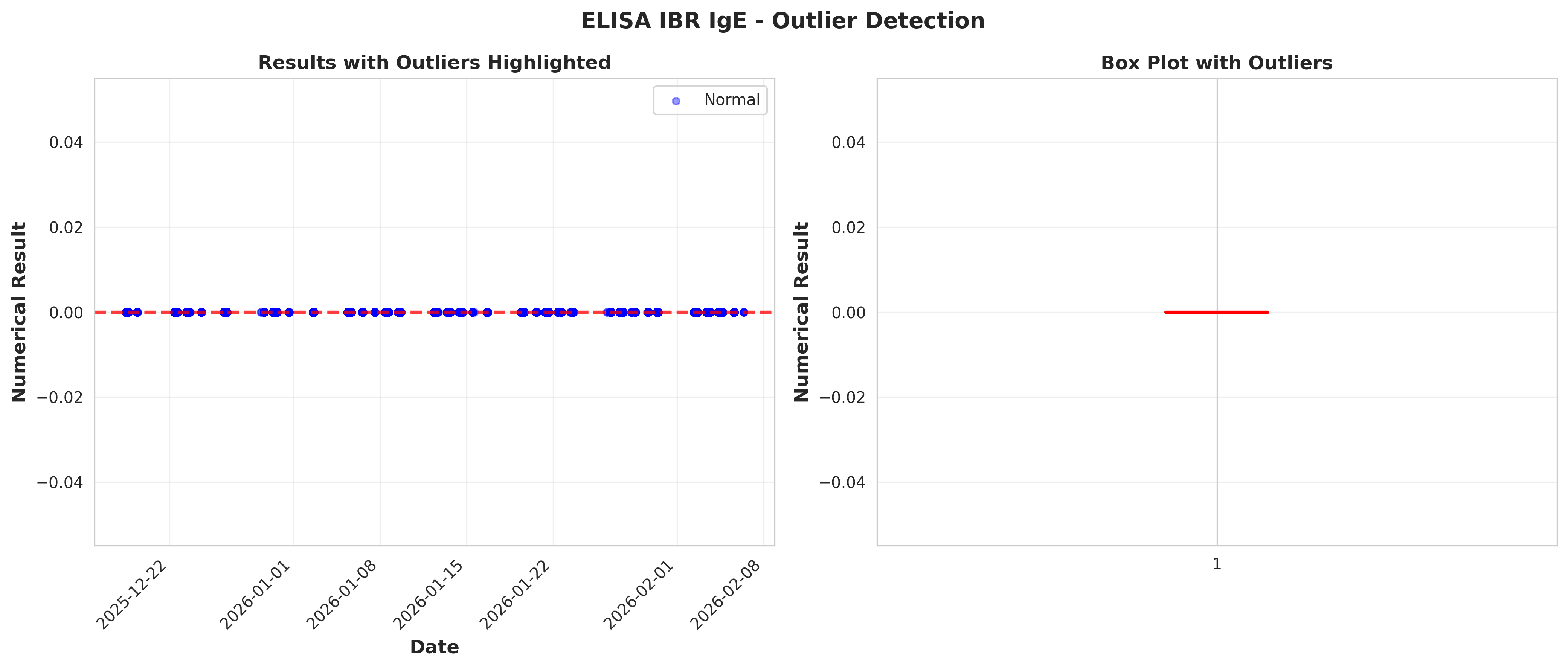
# ========================================================================
# ANALYSIS 4: OUTLIER DETECTION
# ========================================================================
print("\n" + "="*80)
print("ANALYSIS 4: OUTLIER DETECTION")
print("="*80)
# IQR method
Q1 = df_ibr['NumericalResult'].quantile(0.25)
Q3 = df_ibr['NumericalResult'].quantile(0.75)
IQR = Q3 - Q1
lower_bound = Q1 - 1.5 * IQR
upper_bound = Q3 + 1.5 * IQR
outliers = df_ibr[(df_ibr['NumericalResult'] < lower_bound) |
(df_ibr['NumericalResult'] > upper_bound)]
print(f"\nOutlier Detection (IQR method):")
print(f" Lower bound: {lower_bound:.2f}")
print(f" Upper bound: {upper_bound:.2f}")
print(f" Number of outliers: {len(outliers)} ({len(outliers)/len(df_ibr)*100:.2f}%)")
conclusions.append("\n" + "="*80)
conclusions.append("4. OUTLIER ANALYSIS")
conclusions.append("="*80)
conclusions.append(f"\nIQR Method:")
conclusions.append(f" - Lower bound: {lower_bound:.2f}")
conclusions.append(f" - Upper bound: {upper_bound:.2f}")
conclusions.append(f" - Number of outliers: {len(outliers)} ({len(outliers)/len(df_ibr)*100:.2f}%)")
conclusions.append(f" - Outliers below lower bound: {len(outliers[outliers['NumericalResult'] < lower_bound])}")
conclusions.append(f" - Outliers above upper bound: {len(outliers[outliers['NumericalResult'] > upper_bound])}")
if len(outliers) > 0:
outliers_summary = outliers[['ResultDate', 'NumericalResult', 'AnalysisType']].copy()
outliers_summary = outliers_summary.sort_values('NumericalResult', ascending=False)
outliers_summary.to_csv('table_07_outliers.csv', index=False)
print(f" Top 5 highest outliers: {outliers['NumericalResult'].nlargest(5).values}")
# Plot 9: Outlier visualization
fig, (ax1, ax2) = plt.subplots(1, 2, figsize=(14, 6))
# Time series with outliers highlighted
ax1.scatter(df_ibr['ResultDate'], df_ibr['NumericalResult'],
alpha=0.4, s=20, color='blue', label='Normal')
if len(outliers) > 0:
ax1.scatter(outliers['ResultDate'], outliers['NumericalResult'],
alpha=0.7, s=50, color='red', marker='x', label='Outliers')
ax1.axhline(upper_bound, color='red', linestyle='--', linewidth=2, alpha=0.5)
ax1.axhline(lower_bound, color='red', linestyle='--', linewidth=2, alpha=0.5)
ax1.set_xlabel('Date', fontsize=12, fontweight='bold')
ax1.set_ylabel('Numerical Result', fontsize=12, fontweight='bold')
ax1.set_title('Results with Outliers Highlighted', fontsize=12, fontweight='bold')
ax1.legend()
ax1.grid(True, alpha=0.3)
plt.setp(ax1.xaxis.get_majorticklabels(), rotation=45, ha='right')
# Box plot with outliers
bp = ax2.boxplot(df_ibr['NumericalResult'], vert=True, patch_artist=True,
boxprops=dict(facecolor='lightblue', alpha=0.7),
medianprops=dict(color='red', linewidth=2),
flierprops=dict(marker='o', markerfacecolor='red',
markersize=8, alpha=0.5))
ax2.set_ylabel('Numerical Result', fontsize=12, fontweight='bold')
ax2.set_title('Box Plot with Outliers', fontsize=12, fontweight='bold')
ax2.grid(True, alpha=0.3, axis='y')
plt.suptitle('ELISA IBR IgE - Outlier Detection',
fontsize=14, fontweight='bold', y=0.98)
plt.tight_layout()
plt.savefig('plot_09_outlier_detection.png', dpi=300, bbox_inches='tight')
plt.close()
print("Plot 9 saved: Outlier detection")
# ========================================================================
# ANALYSIS 5: CORRELATION WITH TIME
# ========================================================================
print("\n" + "="*80)
print("ANALYSIS 5: CORRELATION WITH TIME")
print("="*80)
# Convert dates to numeric for correlation
df_ibr_sorted = df_ibr.sort_values('ResultDate').copy()
df_ibr_sorted['DaysFromStart'] = (df_ibr_sorted['ResultDate'] -
df_ibr_sorted['ResultDate'].min()).dt.days
if len(df_ibr_sorted) > 2:
corr_coef, p_value = stats.pearsonr(df_ibr_sorted['DaysFromStart'],
df_ibr_sorted['NumericalResult'])
print(f"\nPearson Correlation with Time:")
print(f" Correlation coefficient: {corr_coef:.4f}")
print(f" P-value: {p_value:.4f}")
conclusions.append("\n" + "="*80)
conclusions.append("5. TEMPORAL CORRELATION ANALYSIS")
conclusions.append("="*80)
conclusions.append(f"\nPearson Correlation with Time:")
conclusions.append(f" - Correlation coefficient: {corr_coef:.4f}")
conclusions.append(f" - P-value: {p_value:.4f}")
if p_value < 0.05:
if abs(corr_coef) < 0.3:
strength = "weak"
elif abs(corr_coef) < 0.7:
strength = "moderate"
else:
strength = "strong"
direction = "positive" if corr_coef > 0 else "negative"
conclusions.append(f" - Interpretation: Statistically significant {strength} {direction} correlation")
else:
conclusions.append(f" - Interpretation: No statistically significant correlation with time")
# ========================================================================
# FINAL SUMMARY
# ========================================================================
conclusions.append("\n" + "="*80)
conclusions.append("6. SUMMARY AND CONCLUSIONS")
conclusions.append("="*80)
conclusions.append(f"\nKey Findings:")
conclusions.append(f"1. A total of {len(df_ibr)} ELISA IBR IgE tests were analyzed")
conclusions.append(f"2. Testing frequency averaged {daily_freq['TestCount'].mean():.1f} tests per day")
conclusions.append(f"3. Result values ranged from {result_stats['min']:.2f} to {result_stats['max']:.2f}")
conclusions.append(f"4. Mean result value: {result_stats['mean']:.2f} (±{result_stats['std']:.2f})")
conclusions.append(f"5. {len(outliers)} outliers detected ({len(outliers)/len(df_ibr)*100:.1f}% of data)")
# Identify busiest day
busiest_day = dow_freq.idxmax()
conclusions.append(f"6. Busiest testing day: {busiest_day} ({dow_freq[busiest_day]} tests)")
# Identify month with highest/lowest mean
if len(monthly_results) > 0:
highest_month = monthly_results.loc[monthly_results['Mean'].idxmax()]
lowest_month = monthly_results.loc[monthly_results['Mean'].idxmin()]
conclusions.append(f"7. Month with highest mean result: {highest_month['YearMonth']} ({highest_month['Mean']:.2f})")
conclusions.append(f"8. Month with lowest mean result: {lowest_month['YearMonth']} ({lowest_month['Mean']:.2f})")
conclusions.append(f"\nData Quality Notes:")
conclusions.append(f"- All {len(df_ibr)} records had valid numerical results")
conclusions.append(f"- Date range: {(df_ibr['ResultDate'].max() - df_ibr['ResultDate'].min()).days} days")
conclusions.append(f"- Coefficient of variation: {cv:.2f}%")
conclusions.append("\n" + "="*80)
conclusions.append("END OF ANALYSIS")
conclusions.append("="*80)
# Write conclusions to file
with open('conclusions.txt', 'w') as f:
f.write('\n'.join(conclusions))
print("\nConclusions written to conclusions.txt")
# ========================================================================
# FINAL SUMMARY TABLE
# ========================================================================
summary_data = {
'Metric': [
'Total Records',
'Date Range (days)',
'Mean Tests per Day',
'Mean Result Value',
'Median Result Value',
'Std Dev Result Value',
'Min Result Value',
'Max Result Value',
'Number of Outliers',
'Outlier Percentage',
'Coefficient of Variation (%)'
],
'Value': [
len(df_ibr),
(df_ibr['ResultDate'].max() - df_ibr['ResultDate'].min()).days,
f"{daily_freq['TestCount'].mean():.2f}",
f"{result_stats['mean']:.2f}",
f"{result_stats['50%']:.2f}",
f"{result_stats['std']:.2f}",
f"{result_stats['min']:.2f}",
f"{result_stats['max']:.2f}",
len(outliers),
f"{len(outliers)/len(df_ibr)*100:.2f}",
f"{cv:.2f}"
]
}
summary_df = pd.DataFrame(summary_data)
summary_df.to_csv('table_08_analysis_summary.csv', index=False)
print("Summary table saved")
print("\n" + "="*80)
print("ANALYSIS COMPLETED SUCCESSFULLY!")
print("="*80)
print("\nGenerated Files:")
print(" Tables:")
print(" - table_01_daily_test_frequency.csv")
print(" - table_02_weekly_test_frequency.csv")
print(" - table_03_monthly_test_frequency.csv")
print(" - table_04_result_statistics.csv")
print(" - table_05_day_of_week_analysis.csv")
print(" - table_06_monthly_results_summary.csv")
print(" - table_07_outliers.csv")
print(" - table_08_analysis_summary.csv")
print(" Plots:")
print(" - plot_01_daily_test_frequency.png")
print(" - plot_02_weekly_test_frequency_trend.png")
print(" - plot_03_monthly_test_frequency.png")
print(" - plot_04_results_over_time_scatter.png")
print(" - plot_05_result_distribution.png")
print(" - plot_06_rolling_statistics.png")
print(" - plot_07_day_of_week_patterns.png")
print(" - plot_08_monthly_result_trends.png")
print(" - plot_09_outlier_detection.png")
print(" Text:")
print(" - conclusions.txt")
print("\n" + "="*80)
if __name__ == "__main__":
main()Execution Console
SmartStat Analysis Console
Session: 2e127a06-aade-47e2-aaf1-4ed78b66720e
Ready for analysis...